DOI: 10.1534/genetics.110.125542
Bayesian Multiple Quantitative Trait Loci Mapping for Recombinant
Inbred Intercrosses
Zhongshang Yuan,*
,†Fei Zou
†,‡,1and Yanyan Liu*
*School of Mathematics and Statistics, Wuhan University, Wuhan, Hubei 430072, China and†Department of Biostatistics,
‡Carolina Center for Genome Sciences, University of North Carolina, Chapel Hill, North Carolina 27599
Manuscript received November 30, 2010 Accepted for publication February 17, 2011
ABSTRACT
The Collaborative Cross (CC) is a renewable mouse resource that mimics the genetic diversity in humans. The recombinant inbred intercrosses (RIX) generated from CC recombinant inbred (RI) lines share similar genetic structures to those of F2individuals. In contrast to F2mice, genotypes of RIX can be inferred from the genotypes of their RI parents and can be produced repeatedly. Also, RIX mice do not typically share the same degree of relatedness. This unbalanced genetic relatedness requires careful statistical modeling to avoid a large number of false positivefindings. For complex traits, mapping multiple genes simultaneously is arguably more powerful than mapping one gene at a time. In this article, we describe how we have developed a Bayesian quantitative trait locus (QTL) mapping method that simultaneously deals with the special genetic architecture of RIX and maps multiple genes. The performance of the proposed method is evaluated by extensive simulations. In addition, for a given set of RI lines, there are numerous ways to generate RIX samples. To provide a general guideline on future RIX studies, we compare several RIX designs through simulations.
T
HIS study was motivated by the mouse Collaborative Cross (CC) project. As its main thrust, the CC pro-ject seeks to overcome several of the severe limitations of human complex trait studies. One major limitation of such studies is that only the simplest genetic models can be resolved with confidence. Many other models are plausible, but difficult or impossible to resolve. Because it is closely related to humans, the mouse serves as a great model organism for studying human diseases. Most hu-man genes have functional mouse counterparts, and genomes of both organisms are organized similarly. Tra-ditional RI lines are generated by crossing only two in-bred parental strains, resulting in extensive blind spots where a sizable proportion of the genome is identical by decent (IBD) and a low percentage of genetic variation (15%). In contrast, the CC recombinant inbred (RI) lines are derived from a genetically diverse set of eight founder inbred strains (Chesleret al.2008; Iraqiet al.2008). This selection of founder strains was predicted to result in uniform genome-wide high levels of varia-tion. Genetic variation is randomized in the CC lines so that the causal relationships can be established. Another major advantage of the CC mice is that they are retrievable and extensible, which supports data
integration over space and time and at all levels— from molecules and cells to physiological systems and environments.
Recombinant inbred intercross (RIX) panels are created by generating diallel F1progeny from a set of
RI lines. Given a population ofLRI lines, this approach can potentially produce L(L– 1)/2 genetically distinct RIX individuals. Subsets of RIX can be used to evaluate biological predictions of the ways in which an individual would respond to environmental perturbations and provide statistical support for prediction accuracy. Be-cause RI mice are homozygote at each locus, the geno-types of the derivative RIX mice can be imputed in advance from the genotypes of the parental RI lines. RIX mice with identical genotypes can be regenerated whenever needed. Therefore the CC mice provide us with an ideal platform to generate testable hypotheses that can be used for accurate probability-based whole-organism biological predictions. Preliminary data from the CC strains and their derivative RIX progenies are now being generated. Developing appropriate analysis tools for mapping CC data is critical for the success of the CC project.
Though at the individual level, the genome of each RIX mouse has similar genetic structures to those of F2
individuals, statistical analyses for F2 data cannot be
applied directly to RIX data. Backcross or F2 subjects
used in traditional quantitative trait locus (QTL) map-ping have the same genetic relatedness to each other, which may not be the case for RIX data. Some RIX mice
Supporting information is available online athttp://www.genetics.org/ cgi/content/full/genetics.110.125542/DC1.
1Corresponding author:Department of Biostatistics, University of North
Carolina, 4115D McGavran-Greenberg Hall, CB 7420, Chapel Hill, NC 27599. E-mail: [email protected]
may share common parental RI lines, making them more related to each other than the RIX mice that do not share parental RI lines. Past investigations (Tsaih
et al. 2005; Zou et al. 2005) have shown that careful
statistical analyses that correctly handle the unbalanced relatedness in RIX are important to achieve valid results. Over the last decade, mapping genes of human diseases has been an important research area. The vast majority of genes, however, have been limited to simple Mendelian inheritance patterns and well-defined quan-titative traits with relatively large and consistent effects. Recent emphasis has shifted from mapping simple Mendelian traits to complex traits with complex genetic causes. Complex traits have proved far more resistant to genetic analysis. Many available QTL mapping methods map only one or a few QTL at a time and may not be efficient for complex traits. Variable selection methods are useful in selecting variables that are not necessarily individually important but that are, in fact, jointly im-portant. By treating multiple QTL mapping as a model/ variable selection problem (Broman and Speed2002),
forward and stepwise selection procedures have been proposed to search for multiple QTL. Although simple, these methods have limitations, such as uncertainty about the number of QTL and difficulty in assessing the significance of associated tests due to their sequen-tial model building nature. Bayesian QTL mapping methods (Satagopanet al.1996; Sillanpääand Arjas
1998; Stephensand Fisch1998; Yiand Xu2000, 2001;
Hoeschele2007) have been developed, in particular,
to detect multiple QTL by treating the number of QTL as a random variable and modeling it specifically using reversible-jump Markov chain Monte Carlo (MCMC) (Green 1995). Due to the variable dimensionality of
the parameter spaces associated with different models (different numbers of QTL), one must take care of ac-ceptance probabilities for such changes in dimension, which in practice may not be handled correctly (Ven
2004). One leading approach to variable selection in QTL analysis is the Bayesian analysis based on the com-posite model space framework (Godsill 2001, 2003), first introduced by Yi (2004) to the genetic mapping
community. Reversible-jump MCMC (Green1995) and
stochastic search variable selection (SSVS) (Georgeand
McCulloch1993) are special cases of this analysis. An
alternative to variable selection with SSVS is shrinkage methods (e.g., the lasso method of Tibshirani 1996),
which shrink the effects of unimportant variables near zero. The Bayesian shrinkage methods of Xu(2003) and
Wanget al.(2005) place simple normal priors on QTL
effects. While they can be modified easily, the specific priors used in Xu(2003) and Wanget al.(2005) induce
improper posteriors (TerBraaket al.2005).
In this article, for RIX data, we extend thefixed-effect model of Xu (2003) to a mixed-effects model, where
the complex relationship structure among RIX samples is specifically dealt with through random polygenic
effects. To avoid improper posteriors, we apply the prior modification ofterBraaket al. (2005). To the best of
our knowledge, this is the first simultaneous multiple-QTL mapping method specifically designed for RIX data. This article is organized as follows. Instatistical method, we first introduce the RIX experiment, and
then we propose a mixed-effects model and describe a Bayesian variable selection procedure. Insimulation study, extensive simulations are performed to evaluate
the proposed model and to compare several RIX de-signs. Summary comments are given in thediscussion.
STATISTICAL METHOD
In this section, after describing the RIX design, we propose the multiple-QTL model and introduce the Bayesian variable selection procedure.
RIX design:The RIX panel is created as F1progenies
of RI intercross. For LRI lines, a total of L(L – 1) re-ciprocal RIX andL(L–1)/2 nonreciprocal RIX can be generated (see Figure 1 in Zouet al.2005). For simpli-fication and without loss of generality, in the sequel, we consider the nonreciprocal RIX. Let the parental RI lines be RI1, RI2,. . ., RIL, respectively, and denote the
derived RIX from the RIi ·RIj mating as RIXij, where i,j¼1,. . .,Lwithi,jor, alternatively, as RIXk, where k¼1, 2,. . .,L(L–1)/2 for ease of notation. Letn(#L (L–1)/2) be the total number of RIX sampled andpbe the total number of genetic markers. Further, let the phenotypes (the dependent variable) beyi(i¼1,. . ., n) and the discrete marker genotypes bemij(i¼1,. . ., n,j¼1,. . .,p). We setmijto21, 0, and 1, referring to genotypesaa,Aa, andAA, respectively.
Model: It is often acknowledged that quantitative traits are controlled by both major genes and polygenes, that is, genes with intermediate and small effects, re-spectively. The aggregating effect of polygenes may greatly reduce our ability to map major genes if not modeled carefully. Visscher and Haley (1996)
mod-eled polygenic effects for data derived from commonly used experimental crosses. Methods using Wright’s re-lationship matrix to accommodate different correlations between related individuals have also been developed for pedigree data and diallel data (Goldgar 1990; Amos
1994; Zhuand Weir1996; Xu1998).
RIX data can be viewed as the last generation of a large pedigree that originated from a set of inbred founder strains. Therefore, methods for analyzing pedi-gree data can be directly applied. In our model, we as-sume that major QTL and polygenes affect the trait of interest independently, and the aggregating polygenic effect is normally distributed. For simplicity, we assume that all putative QTL are located on markers, a reason-able assumption with dense maps. For sparse maps, we can employ interval mapping ideas of Wanget al.(2005)
and Huanget al.(2010). Specifically, wefit the
yi5m1 Xp
j51
xijaj1wijbj
1X
L
k51
aikak1ei; (1)
where mis the overall mean,ajandbjare the additive and dominant effects of the jth putative QTL with xij 5pffiffiffi2mij and wij ¼ 12 2jmijj, aik is the number of parents of RIXithat are equal to RIk, and the random polygenic effect ak follows Nð0;s2aÞ (k ¼ 1, 2,. . .,L) and the random error ei follows Nð0;s20Þ (i ¼ 1, 2,. . .,n) and they are independent of each other. Let Abe ann·Lmatrix whose (i,k)th element equalsaik. Clearly, PLk51aik[2 for all i ¼ 1, 2,. . .,n since each RIX has two and only two parents. In the model above, we assume that the polygenic effect is additive, which can be easily extended by adding a random dominance polygenic term in model (1).
In the above model, the observed data are y¼ {yi}, marker genotypes M¼ {mij}, and parental RI informa-tion (i.e., matrix A). The unobserved variables include
m; s20; and sa2;the regression coefficientsa¼{aj},b¼
{bj}; and the random effectsa¼{ak}. Below we describe
the prior distributions of the unobserved variables. Prior specifications:
1. Form:p(m)}1.
2. For theaj’s andbj’s:aj Nð0;s2jÞ;bj Nð0;v2jÞ. 3. Fors2
0:pðs20Þ}1=s20. 4. Fors2
a:pðs2aÞ}ðs2aÞ d21:
Further, for hyperparameters s2j andvj2;we assign the following priors:
5. pðs2 jÞ}ðs2jÞ
d21
andpðv2jÞ}ðvj2Þd21: Hered(0,d #1
2) is used to ensure that the posterior distribution is proper (terBraaket al.2005).
Lets2¼ s2
j andv2¼ v2j
o n o
n
.
The specific priors above result in known marginal conditional distributions for all variables; therefore simple Gibbs sampling can be performed, which we describe below.
MCMC algorithm for posterior computation: We first initiatem, a,b,s20;s2a;s2, andv2. Since the joint pos-terior distribution
pm;a;b;a;v2;s2;s20;s2ajy
}pyjm;a;b;a;v2;s2;s20;s2a
pm;a;b;a;v2;s2;s20;s2a
;
where
pyjm;a;b;a;v2;s2;s20;s2a
}s20
2n=2
· exp
( 2
Pn
i51ðyi2m2 PP
j51
xijaj1wijbj
2PL k51aikakÞ
2
2s2 0
)
;
we perform the following Gibbs sampling steps. Super-scripts (t) and (t11) signify the MCMC iteration steps and we sett¼0 for all initial values.
Step 1. Updating m: m(t11) is drawn from the normal
distribution with mean ð1=nÞPni51yi2PPj51½xijajðtÞ1 wijbjðtÞ2
PL
k51aikaðktÞ
and variances20ðtÞ=n:
Step 2. Updatingajandbj(j¼1,. . .,p),aj(t11)is sam-pled from the normal distribution with mean
Pn
i51
xij21
s2ðtÞ 0
s2ðtÞ
j
21Pn
i51
xij yi2mðt11Þ2
PP j51
wijbðjtÞ2
PL k51
aikaðktÞ
2 P l,j
xilaðlt11Þ2
P l.j
xilaðltÞ
and variance
Xn
i51
xij21s
2ðtÞ
0
s2jðtÞ !21
s20ðtÞ;
whilebj(t11)is drawn from the normal distribution with mean
Pn
i51
w2ij1
s2ðtÞ 0 v2ðjtÞ
21Pn
i51
wij yi2mðt11Þ2
PP j51
xijajðt11Þ2
PL k51
aikaðktÞ
2 P
l,j
wilblðt11Þ2
P l.j
wilblðtÞ
and variance
Xn
i51
w2ij1s
2ðtÞ
0
v2jðtÞ
!21 s20ðtÞ:
Step 3. Updatings2
0:The residual variance is sampled from the scale-inverted x2-distribution, Pn
i51ðyi2mðt11Þ2
PP
j51xijaðt1 1Þ
j 2
PL
k51aikaðktÞ2
PP
j51wijbðt1 1Þ
j Þ
2=
x2 n: Step 4. Updating sj2 and vj2 (j ¼ 1,. . .,p), s
2ðt11Þ
j is
sampled from the scale-inverted x2-distribution,
aj2ðt11Þ= x2122d; and v 2ðt11Þ
j is sampled from the scale-inverted x2-distribution,b2ðt11Þ
j = x2122d:
Step 5. Updatingak(k¼1,. . .,L),ak(t11)is drawn from the normal distribution with mean
Pn
i51
a2ik1s 2ðt11Þ 0 s2aðtÞ
21Pn
i51
aik yi2mðt11Þ2 PP j51
xijajðt11Þ
2PP
j51
wijbðjt11Þ2P l,k
ailaðlt11Þ2
P
l.k ailaðltÞÞ
and variance
Xn
i51
a2ik1 s20ðt11Þ
s2aðtÞ !21
Step 6. Updating s2
a, the random effect variance is sampled from the scale-inverted x2-distribution, PL
k51a 2ðt11Þ k = x2L22d:
After this round of sampling, we complete one sweep of the MCMC and are ready to continue our sampling for the next round by repeating steps 1–6 with the new parameter values. When the chain converges, the sam-pled parameters approximately follow the joint poste-rior distribution. For any parameter of interest, one can easily obtain, for example, its posterior means and var-iances from the joint posterior sample.
SIMULATION STUDY
In this section, we ran extensive simulations to evaluate the performance of the proposed Bayesian method.
Speci-fically, we compared the proposed mixed-effects model with the linear regression model, which ignores the poly-genic effect. We also investigated several RIX designs and compared their abilities in mapping major QTL.
Parental RI genotypes were simulated in R/qtl (Bromanet al.2003), from which RIX genotypes and
phenotypes were generated accordingly. For all simu-lations, we set the true population mean (m) and re-sidual varianceðs20Þto 5.0 and 10, respectively. A single chromosome with total length 15 M was simulated, on which 301 evenly spaced markers (resulting in 300 5-cM intervals) are located. The number of QTL sim-ulated was 4 or 11, and their corresponding genetic effects and locations are summarized in Tables 1 and 2. Threes2
a values, 0, 1, and 8, were simulated, repre-senting the situations where no, low, and high poly-genic effects exist, respectively.
From 100 RI parental lines, a total of 5000 unique nonreciprocal RIX can be produced. For a realistic sample size n that we set to 300 unless specified, we considered the following five designs: (1) the complete-pair design, selecting 25 RI lines randomly and gener-ating all 300 possible nonreciprocal RIX; (2) the loop design (a clockwise mating scheme described in Zou
et al.2005), ordering the 100 RI lines randomly to form a circle and then mating each RI line (clockwise) with the next 3 RI lines after it (i.e., RI1mated with RI2, RI3,
and RI4and RI2mated with RI3, RI4, and RI5, and so
on); (3) the50 complete-independent design, ordering the 100 RI lines randomly and mating RI1with RI2, RI3with
RI4, RI5 with RI6, and so on. The maximal number of
RIX that can be generated from this design isL/2. To achieve the sample size of 300, we may alternatively employ (4) thereplicated-complete-independent design, sam-pling six offspring instead of one from each RIi · RIj mating in design 3, or (5) the 300 complete-independent design, generating 300 independent RIX samples from 600 RI lines as in design 3.
For each simulated datum, the MCMC sampler was run for a total of 63,000 cycles. We set the initial values ofm,a, andbto 0. The initial values ofs20; s2a; s2;and v2were all set to 1. We further set
d to 0.001. Thefirst 3000 cycles were discarded as burn-in, and the remain-der of the chain was thinned by keeping 1 of every 50 samples, resulting in a total of 1200 samples for post-MCMC analysis. All the analysis was done in MATLAB and the MATLAB source code is available at http:// bios.unc.edu/fzou/software/BayesianRIX.
We also analyzed each datum with the linear model
yi5m1 Xp
j51
h
xijaj1wijbj i
1ei; (2)
the gold model for RIX data when the true polygenic effect is zero. All the priors in this linear model were set the same as their counterparts in model (1).
Case 1. Four QTL and s2
a 50: Under this setup, we expect model (2) to perform better than the mixed-effects model (1). The question, more specif-ically, concerns how much better the linear model (2) is. Figure 1 displays the posterior mean estimates for one simulated datum. The two models perform nearly the same, indicating very little power loss of the proposed mixed-effects model.
Case 2. Four QTL ands2
a 58:When the polygenic effect is not zero, Zou et al.(2005) and Tsaihet al. (2005)
have shown that linear models that ignore the unbal-anced relatedness of RIX result in high false positive rates. Figure 2 clearly reflects this. The linear model produces large estimated additive effects for many null
TABLE 1
Locations and sizes of the four simulated QTL
QTL no. Position (cM) Additive effect Dominant effect
1 0 2 2
2 250 1 1
3 500 2 0
4 750 0 2
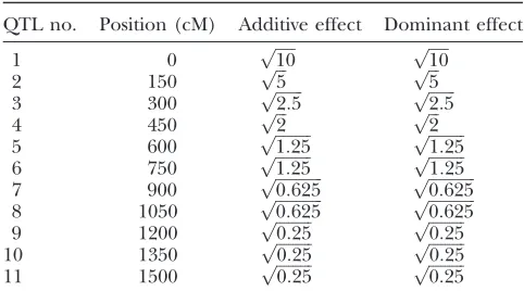
TABLE 2
Locations and sizes of the 11 simulated QTL
QTL no. Position (cM) Additive effect Dominant effect
1 0 pffiffiffiffiffi10 pffiffiffiffiffi10
2 150 pffiffiffi5 pffiffiffi5
3 300 pffiffiffiffiffiffiffi2:5 pffiffiffiffiffiffiffi2:5
4 450 pffiffiffi2 pffiffiffi2
markers. In contrast, the four simulated QTL are map-ped successfully by the mixed-effects model and most of the null markers have their posterior means close to 0. Table 3 shows that for the four simulated QTL, their estimated genetic effects from the mixed-effects model are close to those simulated. The second QTL located at 250 cM is the weakest and its estimated genetic effects depart most from its true genetic values.
In summary, the mixed-effects model performs sub-stantially better than the linear model. Interestingly, there is no significant difference between the two models for detecting dominance effects. This may be attributed to the fact that the simulated polygenic effect is additive, which is less likely confounded with the dominance QTL effects.
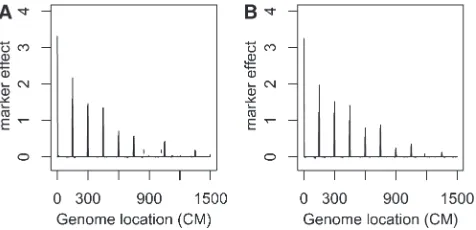
Case 3. Eleven QTL ands2
a51:Under this setup, the heritabilities of 11 QTL decrease from left to right. Figure 3 summarizes the analysis results. The esti-mated genetic effects of the top 6 QTL are signifi -cantly different from 0, and the smallest QTL that the proposed method identified explains 2% of the phenotypic variation.
All the above results are based on data generated from the loop design. Next, we compared the loop design with the other four designs. For each design, we simulated 100 data sets with the genetic configuration from case 2 (i.e., four QTL ands2
a58). The data from the two complete-independent designs were analyzed by the linear model, the correct model for the data. For analysis of the data from the loop, the 300 replicated-complete-independent, and the complete-pair designs, Figure 1.—Bayesian QTL estimates from data simulated
under case 1 where no polygenic effect exists (i.e., s2
a50).
The top two panels are from the linear model, and the bottom two panels are from the proposed mixed-effects model. The height of each vertical line refers the posterior mean estimate of each marker.
Figure 2.—Bayesian QTL estimates from data simulated
under case 2 where polygenic effect existsðs2
a58Þ:The solid lines are for the markers located at the simulated QTL and the dashed lines are for the rest of the markers. See Figure 1 legend for details.
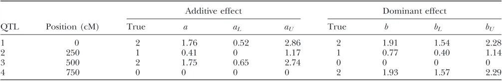
TABLE 3
Estimated QTL effects from data under case 2 with four QTL ands2
a58
Additive effect Dominant effect
QTL Position (cM) True a aL aU True b bL bU
1 0 2 1.76 0.52 2.86 2 1.91 1.54 2.28
2 250 1 0.41 0 1.17 1 0.77 0.40 1.14
3 500 2 1.75 0.65 2.74 0 0 0 0
4 750 0 0 0 0 2 1.93 1.57 2.29
a, posterior mean of additive effect;aLandaU, the 5th and 95th percentiles of posterior samples for the additive effect. Similarly,
we used the mixed-effects model. For the data generated from the 300 replicated-complete-independent design, we also averaged the phenotypes across the six offspring from each RIi · RIj mating and analyzed the 50 in-dependent averages by the linear model. Table 4 sum-marizes the mean squared error (MSE) of the posterior mean estimates of the additive QTL effects. As expected, the data from the 300 complete-independent design perform the best. The loop design is ranked second best and has much higher efficiency than the rest of the designs. Interestingly, though the sample size of the complete-pair design is 300, its power for mapping major QTL is only slightly higher than that of the 50 complete-independent design where the sample size is 50. This is largely due to the fact that we have a large polygenic effect. In summary, for afixed sample size, we recommend sampling as many independent RIX as pos-sible. If the number of independent RIX is too small, the loop design should be our next choice. One advan-tage of the loop design over the independent RIX de-sign is that it allows estimation of the polygenic effect but the independent RIX design does not.
DISCUSSION
Recombinant inbred intercrosses, produced by gener-ating all or a subset of the potential F1hybrids between
pairs of RI lines, increase the number of available
geno-types fromLRI lines toL(L2 1)/2 nonreciprocal RIX and L(L 2 1) reciprocal RIX. Unlike the parental RI lines whose genotypes are homozygous, the genetic struc-ture of RIX resembles that of F2 animals, reducing the
phenotypic anomalies associated with inbred genomes. One of the great achievements of using RIX animals for QTL mapping is the ongoing CC project (Threadgill
et al.2002). The CC project plans to generate and main-tain1000 CC RI lines for scientific research. With such large numbers of RI lines available, our ability to map complex traits can be greatly increased. Because RIX genotypes can be directly inferred from the genotypes of their parental RIs, the genotyping effort required for the CC project is to genotype only the CC RI lines. Fur-ther, due to the renewability of CC mice, new RIX mice can be selectively produced for testing the accuracies of estimated genetic architectures.
In all our simulations, the parameterdis set to 0.001 to ensure a proper posterior distribution. We have also an-alyzed the simulated data withd ¼ 0. The new analysis results are shown insupporting information,File S1, Fig-ure S1, and Figure S2. Though in theory, the posterior distribution from the priors withd¼0 is improper (ter
Braaket al.2005), this adjustment makes very little
dif-ference in practice.
In this article, we have compared several RIX designs. For a given sample size, the complete-independent de-sign performs the best. But the complete-independent design is limited by the number of available RI lines and lacks ability in estimating polygenic effects. In contrast, the loop design and the complete-pair design can generate large numbers of RIX. Between the two, the loop design performs better. We highly recommend the use of the loop design when the number of RI lines is limited. The loop design also provides estimation of polygenic effects for the heritability calculation.
For simplicity, our model assumes no maternal or paternal effects and we consider only nonreciprocal RIX. One major advantage of RIX over RI or F2
pop-ulations is that parent-of-origin effects can be tested with reciprocal RIX. Now we briefly describe how to extend the proposed model for parent-of-origin effects. Figure 3.—Bayesian QTL estimates from data simulated
under case 3. (A) The additive effect; (B) the dominant effect. See Figure 2 legend for details.
TABLE 4
Comparison of thefive designs based on 100 simulations under case 2
Design Position (0 cM) Position (250 cM) Position (500 cM)
300 complete independent 0.17 0.57 0.19
Loop 1.30 0.89 1.46
Replicated complete independenta 3.36 0.94 3.33
Replicated complete independentb 3.45 0.95 3.34
Complete pair 3.50 0.98 3.38
50 complete independent 3.54 1.00 3.58
For each QTL, the mean squared error (MSE) of the posterior mean estimate of the additive effect is reported.
a
Individual phenotypes of RIX samples were analyzed via the proposed mixed-effects model (1).
b
For thejth QTL with additive parent-of-origin effect, we replace the term xijaj in (1) with xij(p)ajp 1 xij(m)ajm,
wherexij(p)[andxij(m)]¼0 or 1 depending on whether
RIXigets an A allele from its father (and mother). Any deviation ofjajp–ajmjfrom 0 suggests a parent-of-origin effect. Polygenic parent-of-origin effects can be similarly modeled. Further, our model basically considers only nucleotide effects, which can be extended as well for modeling founder allelic effects. For example, for the additive effects of the eight CC founder alleles, we can replace the termxijaj1wijbjin (1) withxijbj, wherebj¼ (b1j,. . .,b8j)T and the kth element of xij is 2, 1, or
0 depending on whether RIXiinherits 2, 1, or 0 copies of thekth founder allele (k¼1,. . ., 8) at thejth locus. Therefore,bkjrepresents thekth founder allelic effect. Similarly, for a codominant QTL model, we set bj as a vector of length 36 (corresponding to the 36 geno-types formed by the eight CC founder alleles). We can further treat the QTL effects as random as traditionally done for pedigree data. For example, for an additive model, we let bj Nð0; s2ajIÞ. This would potentially increase the mapping power as the number of param-eters is dramatically reduced.
The authors are grateful for many constructive comments and suggestions from the reviewers and the associate editor. Support for this work was provided in part by National Institutes of Health grants R01GM074175, R01CA082659, and P50MH090338 to F. Zou and grants from the National Science Foundation of China (10771163) and the China Scholarship Council to Z. Yuan and Y. Liu.
LITERATURE CITED
Amos, C. I., 1994 Robust variance-components approach for
assess-ing genetic linkage in pedigrees. Am. J. Hum. Genet.54(3):535– 543.
Broman, K. W., and T. P.Speed, 2002 A model selection approach
for the identification of quantitative trait loci in experimental crosses (with discussion). J. R. Stat. Soc. B64:641–656, 731– 775.
Broman, K. W., H.Wu, S.Senand G. A.Churchill, 2003 R/qtl: QTL
mapping in experimental crosses. Bioinformatics.19:889–890.
Chesler, E. J., D. R.Miller, L. R.Branstetter, L. D.Galloway,
B. L.Jacksonet al., 2008 The Collaborative Cross at Oak Ridge
National Laboratory: developing a powerful resource for systems genetics. Mamm. Genome.19:382–389.
George, E. I., and R. E.McCulloch, 1993 Variable selection via
Gibbs sampling. J. Am. Stat. Assoc.88:881–889.
Godsill, S. J., 2001 On the relationship between Markov chain
Monte Carlo methods for model uncertainty. J. Comput. Graph. Stat.10:230–248.
Godsill, S. J., 2003 Proposal Densities, and Product Space Methods,
in Highly Structured Stochastic Systems. Oxford University Press, London/New York/Oxford.
Goldgar, D. E., 1990 Multipoint analysis of human quantitative
genetic variation. Am. J. Hum. Genet.47:957–967.
Green, P. J., 1995 Reversible jump Markov chain Monte Carlo
com-putation and Bayesian model determination. Biometrika82:711– 732.
Huang, H., H. Zhou, F. Cheng, I. Hoeschele and F. Zou,
2010 Gaussian process based Bayesian semiparametric quantita-tive trait loci interval mapping. Biometrics66:222–232.
Hoeschele, I., 2007 Mapping quantitative trait loci in outbred
pop-ulations, pp. 623–677 in Handbook of Statistical Genetics, Vol. 1, edited byD. J.BALDING, M.Bishopand C.Cannings. John Wiley
& Sons, New York.
Iraqi, F. A., G.Churchilland R.Mott, 2008 The Collaborative
Cross, developing a resource for mammalian systems genetics: a status report of the Wellcome Trust cohort. Mamm. Genome
19:379–381.
Satagopan, J. M., B. S.Yandell, M. A.Newtonand T. C.Osborn,
1996 A Bayesian approach to detect quantitative trait loci using Markov chain Monte Carlo. Genetics144:805–816.
Sillanpaa, M. J., and E.Arjas, 1998 Bayesian mapping of multiple
quantitative trait loci from incomplete inbred line cross data. Genetics148:1373–1388.
Stephens, D. A., and R. D.Fisch, 1998 Bayesian analysis of
quanti-tative trait locus data using reversible jump Markov chain Monte Carlo. Biometrics54:1334–1347.
ter Braak, C. J. F., M. P.Boerand M. C. A. M.Bink, 2005
Ex-tending Xu’s Bayesian model for estimating polygenic effects using markers of the entire genome. Genetics170:1435–1438.
Threadgill, D. W., K. W.Hunterand R. W.Williams, 2002
Ge-netic dissection of complex and quantitative traits: from fantasy to reality via a community effort. Mamm. Genome13:175–178.
Tibshirani, R., 1996 Regression shrinkage and selection via the
lasso. J. R. Stat. Soc. B58:267–288.
Tsaih, S. W., L.Lu, D. C.Airey, R. W.Williamsand G. A.Churchill,
2005 Quantitative trait mapping in a diallel cross of recombinant inbred lines. Mamm. Genome16:344–355.
Ven, R. V., 2004 Reversible-jump Markov chain Monte Carlo for
quantitative trait loci mapping. Genetics167:1033–1035.
Visscher, P. M., and C. S.Haley, 1996 Detection of putative
quanti-tative trait loci in line crosses under infinitesimal genetic models. Theor. Appl. Genet.93:691–702.
Wang, H., Y. M. Zhang, X.Li, G. L.Masinde, S. Mohan et al.,
2005 Bayesian shrinkage estimation of quantitative trait loci pa-rameters. Genetics170:465–480.
Xu, S., 1998 Mapping quantitative loci using multiple families of line
crosses. Genetics148:517–524.
Xu, S., 2003 Estimating polygenic effects using markers of the entire
genome. Genetics163:789–801.
Yi, N., and S.Xu, 2000 Bayesian mapping of quantitative trait loci
under the IBD-based variance. Genetics156:411–422.
Yi, N., and S.Xu, 2001 Bayesian mapping of quantitative trait loci
under complicated mating designs. Genetics157:1759–1771.
Yi, N., 2004 A unified Markov chain Monte Carlo framework for
mapping multiple quantitative trait loci. Genetics167:967–975.
Zhu, J., and B. S.Weir, 1996 Mixed model approaches for diallel
analysis based on a bio-model. Genet. Res.68:233–240.
Zou, F., J. L. Gelfond, D. C. Airey, L. Lu, K. F. Manly et al.,
2005 Quantitative trait locus analysis using recombinant inbred intercrosses (RIX): theoretical and empirical considerations. Ge-netics170:1299–1311.
GENETICS
Supporting Information
http://www.genetics.org/cgi/content/full/genetics.110.125542/DC1
Bayesian Multiple Quantitative Trait Loci Mapping for Recombinant
Inbred Intercrosses
Zhongshang Yuan, Fei Zou and Yanyan Liu
Copyright
©
2011 by the Genetics Society of America
Z. Yuan, F. Zou and Y. Liu 2 SI
FILE S1
Z. Yuan, F. Zou and Y. Liu 3 SI
FIGURE S1.—Bayesian QTL estimates from data simulated under Case 1 where no polygenic effect exists (i.e., 2 = 0). The
parameter was set to 0. The top two panels are from the linear model, where the bottom two panels are from the proposed mixed model. The height of each vertical line refers the posterior mean estimate of each marker.
0 500 1000 1500
0.0
1
.0
2.0
linear model
Genome location (CM)
additiv
e mar
ker eff
e
ct
0 500 1000 1500
0.0
1
.0
2.0
linear model
Genome location (CM)
dominance mar
ker eff
e
ct
0 500 1000 1500
0.0
1
.0
2.0
proposed model
Genome location (CM)
additiv
e mar
ker eff
e
ct
0 500 1000 1500
0.0
1
.0
2.0
proposed model
Genome location (CM)
dominance mar
ker eff
e
Z. Yuan, F. Zou and Y. Liu 4 SI
FIGURE S2.—Bayesian QTL estimates from data simulated under Case 2 where polygenic effect exists (2 = 8). The parameter = 0. See Figure 1 for the figure legends.
0 500 1000 1500
0
.00
.5
1
.01
.5
2
.0
linear model
Genome location (CM)
additiv
e mar
ker eff
e
ct
0 500 1000 1500
0.0
1
.0
2.0
linear model
Genome location (CM)
dominance mar
ker eff
e
ct
0 500 1000 1500
0
.00
.5
1
.01
.5
2
.0
proposed model
Genome location (CM)
additiv
e mar
ker eff
e
ct
0 500 1000 1500
0.0
1
.0
2.0
proposed model
Genome location (CM)
dominance mar
ker eff
e