Please cite this article as: M. Oraon, V. Sharma, Predicting Force in Single Point Incremental Forming by Using Artificial Neural Network, International Journal of Engineering (IJE), IJE TRANSACTIONS A: Basics Vol. 31, No. 1, (January 2018) 88-95
International Journal of Engineering
J o u r n a l H o m e p a g e : w w w . i j e . i rPredicting Force in Single Point Incremental Forming by Using Artificial Neural
Network
M. Oraon*, V. Sharma
Faculty of Production Engineering., Birla Institute of Technology, Mesra, off Campus-Patna Bihar, India
P A P E R I N F O
Paper history:
Received 14 September 2017
Received in revised form 27 October 2017 Accepted 30 November 2017
Keywords:
Single Point Incremental Forming Input variables
ANOVA
Vertical force component Artificial Neural Network
A B S T R A C T
In this study, an artificial neural network was used to predict the minimum force required to single point incremental forming (SPIF) of thin sheets of Aluminium AA3003-O and calamine brass Cu67Zn33 alloy. Accordingly, the parameters for processing, i.e., step depth, the feed rate of the tool, spindle speed, wall angle, thickness of metal sheets and type of material were selected as input and the minimum vertical force component was selected as the model output. To train the model, a Multilayer perceptron neural network structure and feed-forward backpropagation algorithm have been employed. After testing many different artificial neural network (ANN) architectures, an optimal structure of the model i.e. 6-14-1 was obtained. The results, with a correlation relation between experiments to predicted force,-0.215 mean absolute error, show a very good agreement.
doi: 10.5829/ije.2018.31.01a.13
1. INTRODUCTION1
Sheet metals are manufactured by the rolling processes. Sheet metals have various applications starting from a simple sheet metal tray to complicated parts used in aircraft, automotive, construction. The other applications are household appliances, food & beverage containers, boilers, kitchen equipment, office equipment etc. A flat sheet metal is formed into complicated shapes by using the die and punch. The sheet metals are ductile in nature. They can be formed only to a certain limit. Beyond these limit failures like necking and fracture occurs. Many research groups are still investigating process feasibility and developing finite element (FE) codes for the SPIF. Several analysis tools are described in the proceedings [1-4]. Theoretically, the Yielding criteria, strains along with its hardening and thickness variations during the deep drawing of forming process has been established [5] which helps to understand the straining behavior of the thin sheet during incremental sheet metal forming (ISF). In this technique, no need of die and punch as in case of deep drawing. Of course, the deformation is incremental, local in nature and gradual.
*Corresponding Author’s Email:[email protected] (M. Oraon)
These enhance the limiting strain during ISF. It is a growing process; therefore, a wide analysis is required to develop the theory of incremental forming [6, 7]. At present, a number of research works have been carrying out in this field to enhance the process capability of SPIF. The conventional press forming processes become costlier for even small batch production because of the dedicated punch & die, hydraulic press required for forming. In conventional forming, the varying strain path and severe strains reduce the formability of complex shapes. These types of problems can be resolved by using SPIF. Early work in SPIF indicated that the maximum formable wall angle could be a good indicator for material formability [8].
developed on ABAQUS to predict the behaviour of the sheet during ISF to analyse the effect of process parameters like advancing speed, forming in the characteristics of the parts (thickness, geometrical accuracy, roughness) [14]. The formability evaluation on negative ISF has been carried out [15] on pure titanium in cold state ISF [16] and on annealed and pre-aged aluminum AA-2024 grade sheets [17] with varying process parameters. The influence of process parameters on the forming forces have experimentally investigated and analytical results demonstrating the relationship between the respective process parameters and the induced forces [18-22]. An inverse method has been done for adjusting the material parameters for SPIF by FEM simulations called ‘the line test’ on aluminium alloy AA3103 with classical tests and compared with parameters accuracy of the tool force prediction [23] followed by impact of forming parameters on steel DC05 have investigated and confirms forming forces mostly dependent on the size of the wall angle, tool diameter and vertical step sizes of the tool [21]. The constitutive laws (an elastic-plastic law coupled with various hardening models) confirms the thickness of the metal sheet which is a crucial parameters for prediction of an accurate force [24]. Three level box-behnken design of experiments (DOE) approach correlated with quadratic mathematical models for the considered responses i.e. minimizing sheet thinning rate and the punch loads generated in this forming process [25].
2. EXPERIMENTAL INVESTIGATION: MATERIAL, TOOL, AND MACHINE
2. 1. Material The miniaturization trend always finds part with high quality; the body part of aluminium and brass are very demanding in many industries such as aerospace, automobile etc. therefore, commercially available AA 3003-O and calamine brass Cu67Zn33 alloy are taken for experients. The composition of constituents on samples has been found by using scan electron microscopy (SEM). The SEM results shown in Table 1.
The ultimate tensile strength of both metals have been tested on “INSTRON” Series IX automated materials testing system in the department of polymer engineering, Birla Institute of Technology, Mesra. The sample is prepared as per American society for testing’s and materials (ASTM) standard E8 as shown in Figure 1 and corresponding stress-strain curve in Figure 2.
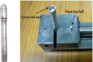
2. 2. Forming Tool A cylindrical rod of 40C6 steel of 07 mm diameter was used as tool. One face of the rod was grooved in such a way that the half part of 06 mm diameter bearing ball inserted in the groove (Figure 3).
TABLE 1. Composition of constituent in AA3003 and
Cu67Zn33 alloy
Constituent (%) AA3003 Cu67Zn33
Al 98.12 -
Si 0.628 -
Fe 0.705 -
Cu 0.05 66.90
Sn - -
Co 0.08 -
Mg 1.2 -
Zr 0.05 -
Zn - 35.06
Pb - 0.01
Figure 1. Samples for ultimate tensile testing of both AA3003
and Cu67Zn33 alloy
Figure 2. Stress-strain curves of test sample of AA3003 and
Cu67Zn33 alloy
Figure 3. Preparation of forming tool and final shape of
Once the bearing ball is worn out due to forming, it can be replaced easily to a new bearing ball which results the saving of new tool preparation and manufacturing cost.
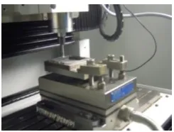
2. 3. SPIF Machine The SPIF is carried out on CNC vertical milling center MIKROTOOLS DT-110 shown in Figure 4 in the Department of Production Engineering, Birla Institute of Technology, Mesra, India. The machine having specifications such as Travel: x-axis: 200 mm, y-axis: 100 mm and z-axis: 100 mm, Spindle speed: 0 -3000, Feed rate: 1-2000 mm/min and Position accuracy: +/-1 micron/100 mm.
3. EXPERIMENTAL DESIGN: DOE
The forces imposed by the tool on the clamped worksheet has been measured through Kistler 9265B six-component force dynamometer shown in Figure 5. It is connected with a multichannel charge amplifier 5017A which have the capacity to measure the three force components i. e. 𝐹𝑥, 𝐹𝑦, and 𝐹𝑧 in the range of -15
to 30 KN. In the present study, the online signals of only vertical force component 𝐹𝑧 captured.
The experiments have been conducted with the aim to identify the relation that exists between each parameter and the minimum veritcal force component 𝐹𝑧. The taghchi design of experiment (DOE) is adopted
for experiments. The experimental set has been designed according to the orthogonal array of 𝐿32 with
two levels.
Figure 4.CNC machine and SPIF set-up for experiment
Figure 5. Arrangement of force dynamometer during
incremental forming
The input parameters 𝑇𝑑, ∆𝑧, 𝑓, 𝑅, 𝜃, 𝑇 and 𝑀 indicates
tool end diameter, step depth, the feed rate of tool RPM, wall angle, the thickness of metal and the types of material respectively. These input variables are chosen for experiemnts based on litrreture review and the level of input variables are set by trail and error pivot experiments. The responses of vertical force component 𝐹𝑧 are shown in Table 2.
4. STATISTICAL ANALYSIS OF THE VERTICAL
FORCE COMPONENT 𝑭𝒛
The statistical analysis is carried out with 95% confidence level by using Minitab 17.0.1 version for finding the significance of input variables. The “smaller is better” approach was chosen because the porpuse is to perform SPIF with low force component 𝐹𝑧.
𝐹𝑧 = −10𝑙𝑜𝑔 1
𝑛 ∑ 𝑦𝑖𝑗2
𝑛
𝑖=1 (1)
where,𝑦𝑖𝑗 is the observed response value.
The tool end diameter 𝑇𝑑 was same for all
experiments, therefore it is kept constant. Figure 6 corresponds to the main response plot for vertical force component 𝐹𝑧. It shows that the suitable combination of
input variables for SPIF with minimum force as ∆𝑧 = 0.1 mm, 𝑓= 20 mm/min, 𝑅 = 2000, 𝜃 = 150, 𝑇 = 0.4 mm, and 𝑀= Cu67Zn33 alloy respectively.
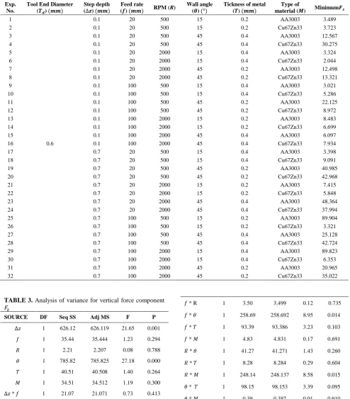
The analysis of variance ANOVA [26] of force component 𝐹𝑧 is tabulated in Table 3. It indicates that
the significance of input variables for SPIF with low force component 𝐹𝑧. Higher significance for SPIF with
low 𝐹𝑧 are found as wall angle 𝜃 (P=0.000) and step
depth ∆𝑧 (P=0.001) whereas other input variables are not significant for the SPIF. As per ANOVA, the SPIF of both materials should be carried out by keeping low wall angle and low step depth. The interaction of input variables i. e. feed rate and wall angle (p= 0.014) and RPM with the types of material (P=0.015) shows their significance for low 𝐹𝑧.
Figure 6. Response of input variables on vertical force
TABLE 2.The input parameters for experiments and output response i.e. vertical force component 𝐹𝑧
Exp. No.
Tool End Diameter
(𝑻𝒅) (𝒎𝒎)
Step depth
(∆𝒛) (𝒎𝒎)
Feed rate
(𝒇) (𝒎𝒎) RPM (𝑹)
Wall angle
(𝜽) (°)
Tickness of metal
(𝑻) (𝒎𝒎)
Type of
material (𝑴) Minimum𝑭𝒛
1
0.6
0.1 20 500 15 0.2 AA3003 3.489
2 0.1 20 500 15 0.2 Cu67Zn33 3.723
3 0.1 20 500 45 0.4 AA3003 12.567
4 0.1 20 500 45 0.4 Cu67Zn33 30.275
5 0.1 20 2000 15 0.4 AA3003 3.324
6 0.1 20 2000 15 0.4 Cu67Zn33 2.044
7 0.1 20 2000 45 0.2 AA3003 12.498
8 0.1 20 2000 45 0.2 Cu67Zn33 13.321
9 0.1 100 500 15 0.4 AA3003 3.021
10 0.1 100 500 15 0.4 Cu67Zn33 5.286
11 0.1 100 500 45 0.2 AA3003 22.125
12 0.1 100 500 45 0.2 Cu67Zn33 8.972
13 0.1 100 2000 15 0.2 AA3003 8.483
14 0.1 100 2000 15 0.2 Cu67Zn33 6.699
15 0.1 100 2000 45 0.4 AA3003 6.097
16 0.1 100 2000 45 0.4 Cu67Zn33 7.934
17 0.7 20 500 15 0.4 AA3003 3.398
18 0.7 20 500 15 0.4 Cu67Zn33 9.091
19 0.7 20 500 45 0.2 AA3003 40.985
20 0.7 20 500 45 0.2 Cu67Zn33 42.968
21 0.7 20 2000 15 0.2 AA3003 7.415
22 0.7 20 2000 15 0.2 Cu67Zn33 5.848
23 0.7 20 2000 45 0.4 AA3003 48.364
24 0.7 20 2000 45 0.4 Cu67Zn33 37.994
25 0.7 100 500 15 0.2 AA3003 89.904
26 0.7 100 500 15 0.2 Cu67Zn33 3.321
27 0.7 100 500 45 0.4 AA3003 25.128
28 0.7 100 500 45 0.4 Cu67Zn33 42.724
29 0.7 100 2000 15 0.4 AA3003 89.823
30 0.7 100 2000 15 0.4 Cu67Zn33 6.353
31 0.7 100 2000 45 0.2 AA3003 20.965
32 0.7 100 2000 45 0.2 Cu67Zn33 35.022
TABLE 3. Analysis of variance for vertical force component
𝐹𝑧
SOURCE DF Seq SS Adj MS F P
∆𝑧 1 626.12 626.119 21.65 0.001
𝑓 1 35.44 35.444 1.23 0.294
𝑅 1 2.21 2.207 0.08 0.788
𝜃 1 785.82 785.825 27.18 0.000
𝑇 1 40.51 40.508 1.40 0.264
𝑀 1 34.51 34.512 1.19 0.300
∆𝑧 * 𝑓 1 21.07 21.071 0.73 0.413
∆𝑧 * 𝑅 1 12.11 12.112 0.42 0.532
∆𝑧 * 𝜃 1 0.35 0.352 0.01 0.914
∆𝑧 * 𝑇 1 48.95 48.953 1.69 0.222
∆𝑧 * M 1 0.92 0.923 0.03 0.862
𝑓 * R 1 3.50 3.499 0.12 0.735
𝑓 * 𝜃 1 258.69 258.692 8.95 0.014
𝑓 * 𝑇 1 93.39 93.386 3.23 0.103
𝑓 * 𝑀 1 4.83 4.831 0.17 0.691
𝑅 * 𝜃 1 41.27 41.271 1.43 0.260
𝑅 * 𝑇 1 8.28 8.284 0.29 0.604
𝑅 * 𝑀 1 248.14 248.137 8.58 0.015
𝜃 * 𝑇 1 98.15 98.153 3.39 0.095
𝜃 * 𝑀 1 0.39 0.387 0.01 0.910
𝑇 * 𝑀 1 7.40 7.401 0.26 0.624
Error 10 289.15 28.915
These input variables must be controlled during the SPIF of aliminum AA3003-O and Cu67Zn33 brass alloy.
5. VALIDATION OF EXPERIMENTAL RESULTS OF FORCE COMPONENT THROUGH ARTIFICIAL NEURAL NETWORK (ANN)
Artificial neural network (ANN) is a computer-based numeric solution for optimisation. ANNs are considered as nonlinear statistical data modeling tools where the complex relationships between inputs and outputs are modeled without having a complete knowledge of relationships between inputs and outputs [27, 28]. However, to generate a valid model, the large amount of data is required for its training and testing, consequently, an extensive period of time is needed for a standard ANN. The better ANN analysis constitutes the network configurations and factors. Therefore, it is required to fix the factors during the investigation. Also, over-fitting should be avoided during the training phase. The dataset for validation (which is independent of the training set) recommended for measuring the error during the analysis. The neural network (NN) stops when the value of error function is minimum (early stopping method).
In the manufacturing process, the output data sets may vary due to assignable causes. Consequently, in ANN, the original dataset putting in training and test sets. Properly trained networks tend to give meaningful answers with inputs parameters that they have never seen. Typically, the introduction of new input leads to an output like the correct output for input vectors used previously in training and that is like the new input being presented. This generalization property makes it possible to train a network on a representative set of input/output pairs and get very good results without training the network on all possible input/output pairs.
A variety of ANN network algorithms has been proposed by researchers for the modeling purpose such as Elman BP, Time-delay BP, Cascade-forward BP, Radial Basis, Self-Organizing Map, and Perception. The feed forward back propagation (FFBP) algorithm [29-32] is widely utilized by investigators for the prediction of surface roughness in SPIF. The BPNN is also applied by the researchers in different manufacturing field such as milling, cutting, turning operations, even in hardness of Al2024-multiwall carbon nano tube [33] for finding the error such as mean square error (MSE), mean absolute error (MAE),root mean square error (RMSE) etc.
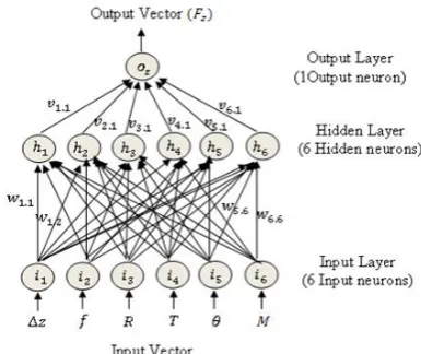
For the present research work, feed forward (FF) neural network structure 6-6-1 is developed (Figure 7). The sigmoidal transfer used for hidden layer neurons whereas the linear activation function used for output.
Figure 7. Structure of 6-6-1 feed-forward network
A three-layer feed-forward network with sigmoid hidden neurons and linear output neurons is developed by using MATLAB, version 7.10.0.499 (R2010a) (Figure 8). Two stopping criteria has been adopted, i.e., sufficient accuracy on the test set and the maximum number of iteration (the first activated).
The ANN model adopted for the present study is summarised below.
5. 1. A Network Model for 𝑭𝒛: Network Algorithm:
FFBP
Training: Levenberg Marquardt (LM) No. of layers: 3
Output: 1
No of neurons : 0 to10
Performance: Mean square error (MSE) Training function: TRAINLM
Hidden layer transfer function: Tran sigmoid Output layer transfer function: Pure linear Adaption of learning rate: LEARNGDM
Figure6 shows the single-layered feed forward (FF) network with one hidden layer. The input to unit𝑥 in hidden layer is expressed in Equation (2),
𝑛𝑒𝑡_ℎ𝑖𝑑𝑑𝑒𝑛 = ∑𝑗𝑗=1𝑤𝑗,𝑥𝑖𝑗+ 𝑏𝑥 (2)
where, 𝑤𝑗,𝑥 is the weight between the input and hidden
neurons and𝑖𝑗 represents the value of the input which
considered for SPIF (Table 3). 𝑏𝑥 represents the biases
on the hidden nodes.
Figure 8. Architecture of two-layer BPNN for surface
The net input to unit 𝑧 in the output layer is expressed in Equation (3):
𝑛𝑒𝑡_𝑜𝑢𝑡𝑝𝑢𝑡 = ∑𝑥𝑥=1𝑣𝑥,𝑧ℎ𝑥+ 𝑐𝑧 (3)
where, 𝑣𝑥,𝑧is the weight between hidden and output
neurons, ℎ𝑥is the value of the output for hidden nodes,
and 𝑐𝑧 represents the biases on the output nodes.
From the output for hidden nodes (Equation (3)) obtained by resolving Equations (2) and (3):
ℎ𝑘= 𝑓(𝑛𝑒𝑡_ℎ𝑖𝑑𝑑𝑒𝑛) (4)
Finally, the output for output nodes as in Equation (5):
𝑜𝑧= 𝑓(𝑛𝑒𝑡_𝑜𝑢𝑡𝑝𝑢𝑡) = 𝑅𝑎 (5)
where, 𝑓 is the transfer function.
In the present study, the hyperbolic tangent sigmoid transfer function (Tansig) and linear transfer function (Purelin) are used at hidden layer and output layer respectively. The 𝑅𝑎 obtained from each experiment are
taken as output whereas different combinations of input parameters (Table 4) are considered as input for predicting surface roughness through ANN. Randomly, the 60% of experimental data are used for training whereas 20% data are used for testing and rest 20% are used for validation of the BP model without normalizing the input data.
6. RESULTS AND DISCUSSION
The output 𝐹𝑧 obtained from experiments of various
combinations was taken as input for the development of BPNN. The predicted 𝐹𝑧 from the NN has been
compared with the experimental 𝐹𝑧. The 60% of whole
data was used for training. The training stopped after 5 iterations. The result is shown in Figure 9. It indicated that the train data best validated at epoch 5 with a value 360.7869.
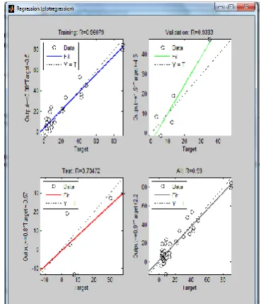
Finally, putting the entire data set through the network (training, validation, and test) and performed a linear regression between the network outputs. The outputs are shown in Figure 10. It seems that the input data for NN is to track the targets reasonably well. The training data set of accuracy 0.960, test data set of 0.704 and validation data set of 0.938 achived through ANN. The overall R-value comes as 0.93. It shows that by using LM algorithm performance of the neural network R-value after simulation comes as 0.93%.
The minimum force 𝐹𝑧 of each experiment was
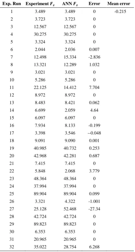
treated as input data for training, test, and validation in the BPNN. The predicted 𝐹𝑧 and corresponding error
presented in Table 4. The predicted 𝐹𝑧 through ANN is
found very close to the experimental data set and found the MAE of -0.215.
Figure 9. Performance plot of back propagation neural
network
Figure 10. Regression plot of back propagation neural
network
7. CONCLUSION
The prediction of process limits in SPIF is very difficult since many variables are involved. Although it is characterized by a localized deformation, the experiments show different process performances, depending on the process parameters. For this reason, during the last decades, several studies, considering this specific process, have been carried out. On the other hand, the achievement of desired surface roughness with SPIF is a major issue.
Optimal designing of the tool and application of suitable input parameters improves the quality of the finished part with low 𝐹𝑧. The selection of desired
TABLE 4. Comparision of experimental and predicted 𝐹𝑧
Exp. Run Experiment 𝑭𝒛 ANN 𝑭𝒛 Error Mean error
1 3.489 3.489 0 -0.215
2 3.723 3.723 0
3 12.567 12.567 0
4 30.275 30.275 0
5 3.324 3.324 0
6 2.044 2.036 0.007
7 12.498 15.334 -2.836
8 13.321 12.289 1.032
9 3.021 3.021 0
10 5.286 5.286 0
11 22.125 14.412 7.704
12 8.972 8.972 0
13 8.483 8.421 0.062
14 6.699 2.059 4.64
15 6.097 6.097 0
16 7.934 8.133 -0.199
17 3.398 3.546 --0.048
18 9.091 9.090 0.001
19 40.985 40.732 0.253
20 42.968 42.281 0.687
21 7.415 7.415 0
22 5.848 2.068 3.779
23 48.364 48.364 0
24 37.994 37.994 0
25 89.904 89.904 0.099
26 3.321 4.322 -1.001
27 25.128 52.468 -27.34
28 42.724 42.724 0
29 89.823 89.823 0
30 6.353 6.353 0
31 20.965 20.965 0
32 35.022 28.754 6.268
So, initial prediction of 𝐹𝑧 in the process will help the
designer to select the best materials and processing technique. In such a condition, the ANN can be a great device which reduces both cost and time. The prediction of any output without conducting the experiments can be done with the help of ANN by adopting previuos experimental data set.
8. REFERENCES
1. Kroplin, B. and Luckey, E., "Metal forming process simulation in industry", in International Conference and Workshop, Baden-Baden, Germany., (1994), 28-30.
2. Lee, J.K., Kinzel, G.L. and Wagoner, R.H., "Numerical simulation of 3-d sheet metal forming processes: Verification of simulations with experiments, Ohio State University, (1996).
3. Guo, Y., Batoz, J., Naceur, H., Bouabdallah, S., Mercier, F. and Barlet, O., "Recent developments on the analysis and optimum design of sheet metal forming parts using a simplified inverse approach", Computers & Structures, Vol. 78, No. 1, (2000), 133-148.
4. Prasanth, I., Ravishankar, D. and Hussain, M.M., "Analysis of milling process parameters and their influence on glass fiber reinforced polymer composites (research note)", International Journal of Engineering-Transactions A: Basics, Vol. 30, No. 7, (2017), 1074-1081.
5. Arab, N. and Nazaryan, E., "Analytical modeling of axi-symmetric sheet metal forming", International Journal of Engineering, Vol. 24, No. 1, (2011).
6. Pohlak, M., Majak, J. and Küttner, R., "Manufacturability and limitations in incremental sheet forming", Proc. Estonian Acad. Sci. Eng, Vol. 13, No. 2, (2007), 129-139.
7. Oraon, M. and Sharma, V., "Sheet metal micro forming: Future research potentials", Int. J. on Production and Industrial Engineering, Vol. 1, No. 01, (2010), 31-35.
8. Jeswiet, J., Micari, F., Hirt, G., Bramley, A., Duflou, J. and Allwood, J., "Asymmetric single point incremental forming of sheet metal", CIRP Annals-Manufacturing Technology, Vol. 54, No. 2, (2005), 88-114.
9. Shim, M.-S. and Park, J.-J., "The formability of aluminum sheet in incremental forming", Journal of Materials Processing Technology, Vol. 113, No. 1, (2001), 654-658.
10. Kim, Y. and Park, J., "Effect of process parameters on formability in incremental forming of sheet metal", Journal of Materials Processing Technology, Vol. 130, (2002), 42-46.
11. Ceretti, E., Giardini, C. and Attanasio, A., "Experimental and simulative results in sheet incremental forming on cnc machines", Journal of Materials Processing Technology, Vol. 152, No. 2, (2004), 176-184.
12. Kopac, J. and Kampus, Z., "Incremental sheet metal forming on cnc milling machine-tool", Journal of Materials Processing Technology, Vol. 162, (2005), 622-628.
13. Obikawa, T., Satou, S. and Hakutani, T., "Dieless incremental micro-forming of miniature shell objects of aluminum foils",
International Journal of Machine Tools and Manufacture, Vol. 49, No. 12, (2009), 906-915.
14. Cerro, I., Maidagan, E., Arana, J., Rivero, A. and Rodriguez, P., "Theoretical and experimental analysis of the dieless incremental sheet forming process", Journal of Materials Processing Technology, Vol. 177, No. 1, (2006), 404-408.
15. Hussain, G., Gao, L. and Dar, N., "An experimental study on some formability evaluation methods in negative incremental forming", Journal of Materials Processing Technology, Vol. 186, No. 1, (2007), 45-53.
16. Hussain, G., Gao, L. and Zhang, Z., "Formability evaluation of a pure titanium sheet in the cold incremental forming process",
The International Journal of Advanced Manufacturing Technology, Vol. 37, No. 9, (2008), 920-926.
17. Hussain, G., Gao, L., Hayat, N. and Dar, N., "The formability of annealed and pre-aged aa-2024 sheets in single-point incremental forming", The International Journal of Advanced Manufacturing Technology, Vol. 46, No. 5, (2010), 543-549. 18. Jeswiet, J., Duflou, J.R. and Szekeres, A., "Forces in single point
and two point incremental forming, Trans Tech Publ, Vol. 6, (2005).
incremental forming", Journal of Materials Processing Technology, Vol. 189, No. 1, (2007), 65-72.
20. Szekeres, A., Ham, M. and Jeswiet, J., "Force measurement in pyramid shaped parts with a spindle mounted force sensor", in Key Engineering Materials, Trans Tech Publ. Vol. 344, (2007), 551-558.
21. Petek, A., Kuzman, K. and Kopac, J., "Deformations and forces analysis of single point incremental sheet metal forming",
Archives of Materials science and Engineering, Vol. 35, No. 2, (2009), 35-42.
22. Ambrogio, G., Duflou, J., Filice, L. and Aerens, R., "Some considerations on force trends in incremental forming of different materials", in AIP Conference Proceedings, AIP. Vol. 907, (2007), 193-198.
23. Bouffioux, C., Eyckens, P., Henrard, C., Aerens, R., Van Bael, A., Sol, H., Duflou, J. and Habraken, A., "Identification of material parameters to predict single point incremental forming forces", International Journal of Material Forming, Vol. 1, (2008), 1147-1150.
24. Henrard, C., Bouffioux, C., Eyckens, P., Sol, H., Duflou, J., Van Houtte, P., Van Bael, A., Duchene, L. and Habraken, A., "Forming forces in single point incremental forming: Prediction by finite element simulations, validation and sensitivity",
Computational Mechanics, Vol. 47, No. 5, (2011), 573-590. 25. Bahloul, R., Arfa, H. and BelHadjSalah, H., "A study on optimal
design of process parameters in single point incremental forming of sheet metal by combining box–behnken design of experiments, response surface methods and genetic algorithms",
The International Journal of Advanced Manufacturing Technology, Vol. 74, No. 1-4, (2014), 163-185.
26. Modanloo, V. and Alimirzaloob, V., "Investigation of the forming force in torsion extrusion process of aluminum alloy
1050", International Journal of Engineering, Transaction C:Aspetcs, Vol. 30, No. 6, (2017), 20-925.
27. Kechman, V., Learning and soft computing. 2001, MIT USA. 28. Neshat, N., "An approach of artificial neural networks modeling
based on fuzzy regression for forecasting purposes",
International Journal of Engineering-Transactions B: Applications, Vol. 28, No. 11, (2015), 1259.
29. Kalidass, S. and Ravikumarb, T.M., "Cutting force prediction in end milling process of aisi 304 steel using solid carbide tools",
International Journal of Engineering-Transactions A: Basics, Vol. 28, No. 7, (2015), 1074-1081.
30. Ambrogio, G., Filice, L., Guerriero, F., Guido, R. and Umbrello, D., "Prediction of incremental sheet forming process performance by using a neural network approach", The International Journal of Advanced Manufacturing Technology, Vol. 54, No. 9, (2011), 921-930.
31. Vahdati, M., Sedighi, M. and Mahdavinejad, R., "Prediction of applied forces in incremental sheet metal forming (ismf) process by means of artificial neural network (ANN)", Journal of Automotive and Applied Mechanics, Vol. 2, No. 2, (2014).
32. Varthini, R., Gandhinathan, R., Pandivelan, C. and Jeevanantham, A.K., "Modelling and optimization of process parameters of the single point incremental forming of aluminium 5052 alloy sheet using genetic algorithm-back propagation neural network", International Journal of Mechanical And Production Engineering, Vol. 2, No. 5, (2014), 55-62. 33. Jafari, M.M. and Khayati, G.R., "Artificial neural network based
prediction hardness of al2024-multiwall carbon nanotube composite prepared by mechanical alloying", International Journal of Engineering, Transaction C: Aspetcs, Vol. 29, No. 12, (2016), 1726-1733.
Predicting Force in Single Point Incremental Forming by Using Artificial Neural
Network
M. Oraon, V. Sharma
Faculty of Production Engineering., Birla Institute of Technology, Mesra, off Campus-Patna Bihar, India
P A P E R I N F O
Paper history:
Received 14 September 2017
Received in revised form 27 October 2017 Accepted 30 November 2017
Keywords:
Single Point Incremental Forming Input variables
ANOVA
Vertical force component Artificial Neural Network
ديكچ ه رد نیا ،هعلاطم کی هکبش یبصع یعونصم یارب شیپ ینیب لقادح یورین دروم زاین یارب لیکشت کت هلحرم یا ( SPIF ) قرو یاه کزان موینیمولآ AA3003-O و ژایلآ Cu67Zn33 جنرب Calamine دروم هدافتسا رارق تفرگ . رب نیا ،ساسا یاهرتماراپ ،شزادرپ هب ناونع ،لاثم قمع ،مدق تعرس هیذغت ،رازبا تعرس ،رشاو هیواز ،راوید تماخض قرو یاه یزلف و عون داوم باختنا هدش هب ناونع یدورو باختنا دش و لقادح یازجا یورین یدومع هب ناونع یجورخ لدم باختنا دش . یارب شزومآ ،لدم راتخاس هکبش یبصع نترپورپ Multilayer و متیروگلا تشگزاب بقع هب ولج هدافتسا هدش تسا . سپ زا شیامزآ یرایسب زا یرامعم یاه هکبش یاه یبصع یعونصم ( ANN ) ، راتخاس هنیهب یا زا لدم 6 -14 -1 تسدب دمآ . ،جیاتن اب کی هطبار یگتسبمه نیب شیامزآ اه هب یورین شیپ ،ینیب -0.215 نیگنایم یاطخ ،قلطم ناشن یم دهد هک قفاوت رایسب یبوخ تسا .