80 Trans. Phenom. Nano Micro Scales, 7(2): 80-87, Summer and Autumn 2019 DOI: 10.22111/tpnms.2018.17962.1107
Sensitivity analysis of the effective nanofluid parameters flowing in flat tubes
using the EFAST method
Moein Taheri1, Hamed Safikhani1,*, Mostafa Usefi2
1Department of Mechanical Engineering, Faculty of Engineering, Arak University, Arak, Iran 2Department of Mechanical Engineering, Faculty of Engineering, University of Guilan, Rasht, Iran
Received 27 November 2016; revised 1 November 2018; accepted 11 November 2018; available online 29 July 2019
ABSTRACT: In the present study, the effective parameters of water-Al2O3 nanofluid flowing in flat tubes are investigated using the
EFAST Sensitivity Analysis (SA) method. The SA is performed using GMDH type artificial neural networks (ANN) which are based on validated numerical data of two phase modeling of nanofluid flow in flat tubes. There are five design variables namely: tube flattening (H), flow rate (Q), wall heat flux (q"), nanoparticle diameter (dp) and nanoparticle volume fraction (φ) and there are two objective functions namely: pressure drop (∆P) and heat transfer coefficient (h). The results show that among design variables, the tube flattening has the highest effect on variations of pressure drop (74%) and heat transfer coefficient (40%). Except tube flattening, the flow rate and the nanoparticle volume fraction has the highest effect on pressure drop (24%) and heat transfer coefficient (25%) respectively. The effects of all of the design variables on objective functions are shown in the results.
KEYWORDS: EFAST method; flat tubes; nanofluid; Sensitivity analysis
INTRODUCTION
One of the applicable techniques for heat transfer augmentation is the use of Nanofluid. Nanofluid have attracted enormous interest from researchers due to high thermal conductivity and their potential for high rate of heat exchange incurring little penalty in pressure drop. Since a decade ago, research publications related to the use of nanofluid as working fluids have been reported both experimentally and numerically.
Razi et al. [1] investigated a CuO-Oil mixture experimentally in different flat tubes and finally presented correlations for defining the Nusselt number and pressure drop of nanofluid flow in the flat tubes.
Murshed et al. [2] carried out an experimental work, which has been considered the effects of particle size, nanolayer, Brownian motion and particle surface chemistry and interaction potential on the thermal conductivity of nanofluid and proposed a new model for thermal conductivity. Besides experimental studies Computational Fluid Dynamics (CFD) has a great potential to predict the fluid dynamics and heat transfer performance of nanofluid. Shariat et al. [3] used two phase mixture model to simulate the nanofluid flow in different horizontal tubes with elliptical sections.
They simulated laminar and mixed convection flow and discussed the effect of parameters such as Richardson number and particle size on the flow field.
*Corresponding Author Email: [email protected]
Tel.: +989120686211; Note. This manuscript was submitted on November 27, 2016; approved on November1, 2018; published online July 29, 2019.
Akbarinia and Laur [4] studied the effect of nanoparticles diameter on nanofluid in horizontal curved tubes with circular cross section using two phase mixture model. Kalteh et al. [5] studied the forced laminar convection nanofluid flow in a rectangular microchannel using two phase Eulerian-Eulerian approach.
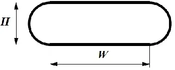
Another technique which is employed to enhance heat transfer is the use of flat tubes in heat exchangers. Flat tubes are geometrical modified round tubes which can be manufactured by flattening the round tubes into an oblong shape. Figure 1 shows the schematic of a flat tube cross section.
Fig. 1. Geometry cross section of a flat tube
81
Nomenclature
a Acceleration (m s-2) W Width of flat tubes (mm)
Cd Dispersion coefficient
Cf Skin friction coefficient Greek symbol
Cp Specific heat (J kg -1
K-1) α Thermal diffusivity
dp Diameter of nanoparticles (m) β Volumetric expansion coefficient (K
-1
)
g Gravitational acceleration (m s-2) δ Distance between particles (m)
h Heat Transfer coefficient (W m-2 K-1)
Nanoparticles volume fractionH Internal Height of Flat tube (mm) μ Dynamic viscosity (N s m-2)
k Thermal conductivity (W m-1 K-1) ρ Density (kg m-3)
kB Boltzmann constant (=1.3807
10-23
J K-1) w Wall shear stress (Pa)
Nu Nusselt Number (=hDh/k) Subscripts
P Perimeter of flat tubes (mm) dr Drift
Q Volumetric flow rate (m3/ hr) f Fluid
q Heat flux (W m-2) i Inlet conditions
Re Reynolds number (=VDh/νm) m Mixture
T Temperature (K) p Nanoparticle phase
V Velocity (m s-1) w Wall
of heat transfer augmentation. Shah and London [6] summarized many analytical and some experimental results for laminar flow characteristics and heat transfer with a single-phase fluid in flat tubes. Vajjha et al. [7] used single phase approach to simulate the fluid dynamics and heat transfer performance of different nanofluid in a single flat tubes of an automobile radiator. They used convection coefficient for the wall boundary condition and finally presented the correlation for local Nusselt number and friction factor of the automobile flat tube. Safikhani and Abbassi [8] investigated the effect of tube flattening in flat tubes containing nanofluid using CFD techniques. Safikhani et al [9] performed multi-objective optimization of nanofluid flow in flat tubes using combination of CFD, GMDH artificial neural networks and NSGA II algorithm. The GMDH polynomials presented by Safikhani et al. [9] will be used in the present study for sensitivity analysis of nanofluid floe in flat tubes.
Both the heat transfer coefficient ( ̅) and the pressure drop (∆P) in different heat exchangers are two important objective functions to be analyzed using sensitivity analyses method. Based on our information, no sensitivity analysis research has been carried out so far on nanofluid flow in flat tubes.
Therefore, sensitivity analysis is investigated in the present study by using the EFAST method.
Sensitivity analysis refers to the study of “how uncertainty in model output (numerical and non-numerical) can be classified into different sources of uncertainty in model input factors.” [10]. Saltelli et al. [11] have classified the sensitivity analysis methods into two groups: local and general.
The local sensitivity analysis methods analyze the response of model output(s) by changing one of the parameters and maintaining the other parameters at central values; while the general sensitivity analysis methods investigate the general response of model output(s)
(averaged over the variation of all the parameters) by searching a finite (or infinite) region. Although the local sensitivity analysis method is simple to use, it just analyzes one point at a moment; so nowadays, the general sensitivity analysis methods are preferred to the local ones.
As was mentioned, sensitivity analysis can specify the sensitive and insensitive parameters of a model. In this regard, Korayem et al. [12] investigated the use of different contact models in the AFM-based manipulation of biological cells in bio-environments.
They employed the Sobol method to analyze the sensitivity of the modeling parameters of 4 contact mechanics models (PT, Hertz, DMT and JKR). Hertz model is very sensitive to the Young’s modulus , and the sensitivity of the adhesion energy in this model is zero (Hertz model disregards the effect of adhesion energy). Contrary to Hertz model, the other three models are highly sensitive to the adhesion energy as well as the elasticity modulus.
All the models show little sensitivity to the parameters of particle radius and Poisson’s ratio.
Based on our information, no sensitivity analysis research has been carried out so far on nanofluid flow in flat tubes.
Therefore, sensitivity analysis is investigated in the present study using the EFAST method.
DEFINING THE DESIGN VARIABLES
The design variables in the present study are: tube flattening (H), inlet volumetric flow rate (Qi), wall heat flux
( ), nanoparticle diameter (dp) and nanoparticle volume
fraction (Φ).
82 Table 1
Design variables and their range of variations. Design Variables
From To
H(mm) 2 10
Qi(m3/hr) 0.002826 0.014130
(kw/m2) 1 5
Φ(%) 0 5
dp(nm) 20 100
About the tube flattening (geometry) it should be mentioned that the same perimeter is a constraint which was observed by the other researchers who have studied the flat tubes [1, 8 and 19].
It is evident that since the perimeter of tubes are constant, the H and W parameters in Figure 1 depend on each other and if one of them is known, the other one could be calculated with respect to the constant perimeter constraint. Therefore in this paper, “H” is used to define each flat tube. Figure 2 shows three different flat tubes with the same perimeter constraint.
Fig. 2. Dimensions of three flat tube cross sections in the present simulations
Moreover because the hydraulic diameter of tubes are different, the design variables and objective function should not be presented in the non-dimensional form [1,8,19], therefore instead of using non-dimensional parameters such as Nu, Re, Cf and Gr, their associated dimensional
parameters h, Qi, τw and are used. The sensitivity
analysis in the present paper is performed using the GMDH type Artificial Neural Network (ANN) models and CFD data which were presented in [9].
CFD AND GMDH TYPE ANN MODELS
The sensitivity analysis (SA) presented in this paper is performed using GMDH type artificial neural networks (ANN) which are based on validated numerical data of two phase mixture modeling of nanofluid flow in flat tubes. The
details of numerical modeling and GMDH polynomials are presented in [9]. The details of dimensions and operating conditions are shown in Table 2 and moreover a sample of numerical simulation which presents the details of temperature contours in different flat tubes is shown in Figure 3. In the present study, numerical simulation of nanofluid flow is performed using mixture model which is a single fluid two phase approach. In this method each phase has its own velocity field, and in a given control volume there is a certain fraction of base fluid and nanoparticles. Instead of utilizing the governing equations of each phase separately, it solves the continuity, momentum and energy equations for the mixture, and the volume fraction equation for nanoparticles. A second order upwind method is used for the convective and diffusive terms and the SIMPLE algorithm is employed to solve the coupling between the velocity and pressure fields. Constant velocity and temperature in inlet, constant wall heat flux in walls and fully thermally and hydro dynamically boundary conditions are used.
Fig. 3. Effect of tube flattening on fully developed temperature contours
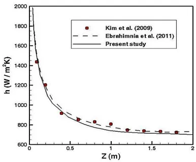
To attain confidence about the simulations, it is necessary to compare the simulation results with the available data.
Figure 4 compares the local heat transfer coefficient for a circular tube of present study with the experimental study carried out by Kim et al. [14] and numerical study of Ebrahimnia et al. [15]. As is evident from this figure the present simulations agree well with the available experimental and numerical data.
SENSITIVITY ANALYSIS METHODS
83
Fig. 4. Comparison of the local heat transfer coefficient with the measured data
The general sensitivity analysis methods are
implemented in four steps: (1) defining the inputs and the type of distribution of each input, (2) generating the samples for the input values, (3) computing the model’s output for each set of input samples and (4) determining the effect of each input factor on the output [16]. In this section, the variance-based sensitivity analysis methods have been reviewed. The variance-based general sensitivity analysis approaches can be used to obtain the first-order effect and the second-order effect (which include the interaction between other parameters) [17].
The Sobol method [18] is a model-independent general sensitivity analysis method which is based on variance analysis.
This method can be used for nonlinear and non-uniform functions and models. For the model defined by function Y=f(X), where Y is the model output and X(X1,X2,…,Xn) is
the vector of input parameters, Sobol suggested to decompose the function f into summands of increasing dimensionality, where the integral of each term over its own input variables is zero.
Sobol showed that, when all the inputs are perpendicular to one another, this resolution is unique and the output variance of the model (V) is the set of variances of each resolved term [18]:
n n n j i ij n i
i V V
V Y
V 1...
1 ... ) (
(1)In relation1, Vi denotes the first-order effect for each
input factor xi(Vi=V[E(Y|xi)]), and Vij(Vij=V[E(Y|xi,xj)]-Vi
-Vj) to V1,…,n indicate the interactions between n factors.
Therefore, the shares allocated to parameters, and the interactions of parameters can be determined from the total output variance.
The sensitivity index is obtained as the ratio of each order’s variance to the total variance (Si=Vi/V) denotes the
first-order sensitivity index, Sij=Vij/V represents the
second-order sensitivity index, and so on).
The total sensitivity index (i.e., the overall effect of each parameter) is obtained as the summand of all the orders of sensitivity index for that parameter [18]:
j i ij iTi
S
S
S
(2)The EFAST method was presented by Cukier et al. [19] and was later improved by Saltelli et al. [20]. Like the Sobol method, this approach is also based on variance and it is independent of any assumption of linearity and uniformity between inputs and output(s).
Contrary to the Sobol method, which uses
multidimensional integrals to obtain the total variance and
the partial variances, this method converts the
multidimensional integrals to one-dimensional ones by defining a transfer function and simplifies the procedure for the calculation of sensitivity indexes.
The EFAST method searches the n-dimensional space of the input factors (Unit Hypercube Kn) by using a Search Curve defined by a set of parametric equations [20]:
i i
i
s
x
1
arcsin
sin
2
1
(3)
Where ωi(i=1,2,…,n) is the frequency related to factor xi,
s is a variable that changes from –π to +π, and φi specifies
the starting point of the curve. The output variance of the model is approximated by means of Fourier analysis:
2 2)
(
2
1
)
(
2
1
ds
s
f
ds
s
f
Y
V
j jj
B
A
B
A
)
(
)
(
2 2 02 02
N j j j B A 1 2 2 ) ( 2 (4)
In the above relation, f(s)=f(G1(sin(ω1s)),
G2(sin(ω2s)),…,Gn(sin(ωns))),G(s) are the transfer
functions, and Aj and Bj are the Fourier coefficients
(Aj= ∫ ∫ . By
calcu-ting the Fourier cofficients for the basic frequency (ωi) and its higher harmonics (pωi), the partial first-order
input variance (xi) can be obtained.
0 1 2 2 22 ) 2 ( )
( Z p p p p p p
i A i B i A i B i
V (5)
Also, like the Sobol method, the ratio of the first-order partial variance to total variance is used to compute the main sensitivity index.
84
V
V
ST
ii
1
(6)Variance V-i is obtained by changing all the parameters
except parameter xi.
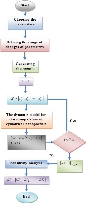
The Sobol method employs the Monte Carlo integral to obtain each partial variance; and in comparison with the EFAST method, it doesn’t use a transfer function; that’s why, it has a low computational efficiency. Algorithm of sensitivity analysis is shown in Figure 5.
RESULTS OF SENSITIVITY ANALYSIS
The results of sensitivity analysis for heat transfer coefficient ( ̅) and the pressure drop (∆P) have been presented in this section. Employing the EFAST method, the sensitivity of five parameters: tube flattening (H), inlet
volumetric flow rate ( ), wall heat flux ( ), nanoparticle
diameter ( ) and nanoparticle volume fraction (Φ), have been explored for heat transfer coefficient ( ̅) and the pressure drop (∆P).
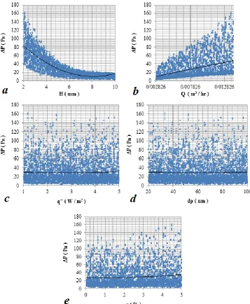
Figure 6a illustrates the changes of the pressure drop with tube flattening. It indicates that, with the increase of this sensitive parameter, the pressure drop diminishes. As is observed in this figure, at low values of tube flattening, sensitivity is greater and with the increase of tube flattening, the slope of the diagram becomes milder. So, by considering the results that indicate the effect of this parameter on the pressure drop, the proper values for this parameter can be selected. Also, in the group of sensitive parameters, the tube flattening parameter has a high sensitivity for the pressure drop. As is shown in Figure 6b, with the increase in the inlet volumetric flow rate, the pressure drop also increases with a very sharp slope. So, the second most sensitive parameter is the inlet volumetric flow rate parameter. The other investigated parameter is the wall heat flux; and considering a near zero slope for the diagram showing the changes of the pressure drop versus wall heat flux (Fig. 6c), this parameter is not considered to be a sensitive parameter either for the pressure drop, and choosing different values for this parameter from its range of changes doesn’t lead to a tangible change in the pressure drop values.
As Figure 6d demonstrates, the diagram showing the changes of the pressure drop versus the nanoparticle diameter selected, has very mild and near zero slopes. This indicates that by altering the values of this parameter in its respective ranges, no substantial change will be induced in the pressure drop.
The diagram of the pressure drop versus nanoparticle volume fraction has been shown in Figure 6e with a positive, and near zero, slope. With the change of nanoparticle volume fraction in its range of variations, a minor change is observed in the pressure drop, and so this parameter is not considered as a sensitive parameter for the pressure drop.
Fig. 5. Algorithm of sensitivity analysis
The changes of the heat transfer coefficient with tube flattening have been shown in Figure 7a.
According to this diagram, with the increase of tube flattening, heat transfer coefficient diminishes. As is observed in this figure, at low values of tube flattening, sensitivity is greater and with the increase of tube flattening, the slope of the diagram becomes milder. So, by considering the results that indicate the effect of this parameter on the heat transfer coefficient, the proper values for this parameter can be selected. Another sensitive parameter among the parameters is the inlet volumetric flow rate.
According to Figure 7b, with the increase of this parameter, the heat transfer coefficient increases with a linear slope. This linear increase indicates that the sensitivity of this parameter is the same in all its range of changes.
85 With the change of wall heat flux in its range of variations, a major change is observed in the heat transfer
coefficient.
Fig. 6. The changes of pressure drop with: (a) tube flattening, (b) inlet volumetric flow rate, (c) wall heat flux, (d) nanoparticle diameter and (e) nanoparticle volume fraction
So, the third most sensitive parameter to which the heat transfer coefficient is sensitive is the wall heat flux. Another sensitive parameter among the input parameters is nanoparticle diameter.
86
Fig. 7. The changes of the heat transfer coefficient with: (a) tube flattening, (b) inlet volumetric flow rate, (c) wall heat flux, (d) nanoparticle diameter and (e) nanoparticle volume fraction
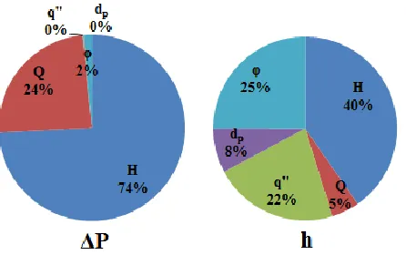
Figure 8 indicates more accurate analysis of the results obtained by the EFAST sensitivity analysis method. According to Figure 8, as expected, tube flattening (with a sensitivity index of 74%), inlet volumetric flow rate (with a sensitivity index of 24%) and nanoparticle volume fraction (with a sensitivity index of 2%), are of most significant sensitivity among five parameters in pressure drop. Also, According to Figure 8, tube flattening (with 40% sensitivity) is the most important parameter, and the parameters of inlet volumetric flow rate and wall heat flux (with 25% and 22% sensitivities, respectively) are the other effective parameters in heat transfer coefficient.
CONCLUSION
In the present study, the effective parameters of water-Al2O3 nanofluid flowing in flat tubes were investigated
87
Fig. 8. Percent sensitivity of input parameter changes in the pressure drop and heat transfer coefficient
The results show that among design variables, the tube flattening has the highest effect on variations of pressure drop (74%) and heat transfer coefficient (40%). Except tube flattening, the flow rate and the nanoparticle volume fraction has the highest effect on pressure drop (24%) and heat transfer coefficient (25%) respectively. The effects of all of the design variables on objective functions were shown in the results (Fig. 8).
REFERENCES
[1] Razi P, Akhavan-Behabadi MA, Saeedinia M.
Press-ure drop and thermal characteristics of CuO–base oil nanofluid laminar flow in flattened tubes under constant heat flux. Int. Commun. Heat Mass Transfer. 2011; 38: 964–71.
[2] Murshed S, Leong K, Yang C. A combined model
for the effective thermal conductivity of nanofluids. Appl. Therm. Eng. 2009; 29: 2477-83.
[3] Shariat M, Akbarinia A, HosseiNezhad A,
Behzadmehr A, Laur R. Numerical study of two phase laminar mixed convection nanofluid in elliptic ducts. Appl. Therm. Eng. 2011; 31: 2348-59. [4] Akbarinia A, Laur R. Investigation the diameter of
solid particles effects on a laminar nanofluid flow in a curved tube using a two phase approach. Int. J. Heat Fluid Flow. 2009; 30(4); 706-14.
[5] Kalteh M, Abbassi A, Saffar-Avval M, Harting J.
Eulerian–Eulerian two-phase numerical simulation of nanofluid laminar forced convection in a microchannel. Int. J. Heat Fluid Flow. 2011; 32:107–16.
[6] Shah RK, London AL. Laminar Flow Forced
Convection in Ducts. Academic Press, New York. 1978.
[7] Vajjha R, Das D, Namburu P. Numerical study of
fluid dynamic and heat transfer performance of Al2O3 and CuO nanofluids in the flat tubes of a
radiator. Int. J. Heat Fluid Flow. 2010; 31: 613–21.
[8] Safikhani H, Abbassi A. Effects of tube flattening on
the fluid dynamic and heat transfer performance of
nanofluid flow. Adv. Powder Technolog. 2014; 25(3):1132-41.
[9] Safikhani H, Abbassi A, Khalkhali A, Kalteh M.
Multi-objective optimization of nanofluid flow in flat tubes using CFD, Artificial Neural Networks and genetic algorithms. Adv. Powder Technolog. 2014; 25(5): 1608-17.
[10] Saltelli A, Sobol IM. About the use of rank
transformation in sensitivity analysis of model
output. Reliability Engineering & System
Safety.1995 ; 50(3) : 225-39
[11] Saltelli A, Chan K, Scott E. Sensitivity analysis Wiley series in probability and statistics. Willey, New York. 2000
[12] Korayem M, Rastegar Z, Taheri M. Sensitivity
analysis of nano-contact mechanics models in manipulation of biological cell. Nanoscience and Nanotechnology. 2012 ; 2(3):49-56.
[13] Quiben J, Cheng L, Da Silva J, Thome J. Flow
Boiling in horizontal flattened tubes: Part I – Two-phase frictional pressure drop results and model. Int. J. Heat Mass Transf. 2009; 52(15-16): 3645-53.
[14] Kim D, Kwon Y, Cho Y, Li C, Cheong S, Hwang Y,
Lee J, Hong D,Moon S. Convective heat transfer characteristics of nanofluids under laminar and turbulent flow conditions. Current Applied Physics. 2009; 9(2): 119-23.
[15] Ebrahimnia-Bajestan E, Niazmand H,
Duangthongsuk W, Wongwises S. Numerical investigation of effectiv parameters in convective heat transfer of nanofluids flowing under a laminar flow regime. Int. J. Heat Mass Transf. 2010; 54 (19-20): 4376-88.
[16] Tong C. Self-validated variance-based methods for
sensitivity analysis of model outputs. Reliability Engineering & System Safety. 2010; 95 (3): 301-9.
[17] Nossent J, Elsen P, Bauwens W. Sobol’sensitivity
analysis of a complex environmental model. Environmental Modelling & Software. 2011; 26(12): 1515-25.
[18] Sobol IM. Sensitivity estimates for nonlinear
mathematical models. Mathematical Modeling and Computational Experiments.1993; 14; 407-14.
[19] Cukier R, Levine H, Shuler K. Nonlinear sensitivity
analysis of multiparameter model systems. Journal of computational physics.1978; 26(1): 1-42.
[20] Saltelli A, Tarantola S, Chan KS. A quantitative model-independent method for global sensitivity analysis of model output. Technometrics. 1999; 41, 39-56.
[21] Homma T, Saltelli A. Importance measures in global