An enhanced training algorithm for multilayer neural networks based on reference output of hidden layer

1999 Springer-Verlag London Limited

An Enhanced Training Algorithm for Multilayer Neural

Networks Based on Reference Output of Hidden Layer

Y. Li

_{, A.B. Rad}

_{and W. Peng}

1_{Department of Electrical Engineering, The Hong Kong Polytechnic University, Kowloon, Hong Kong;} 2_{School of Engineering,} The Flinders University of South Australia, Adelaide, Australia

In this paper, the authors propose a new training algorithm which does not only rely upon the training samples, but also depends upon the output of the hidden layer. We adjust both the connecting weights and outputs of the hidden layer based on Least Square Backpropagation (LSB) algorithm. A set of ‘required’ outputs of the hidden layer is added to the input sets through a feedback path to accelerate the convergence speed. The numerical simulation results have demonstrated that the algorithm is better than conventional BP, Quasi-Newton BFGS (an alternative to the conjugate gradient methods for fast optimisation) and LSB algorithms in terms of convergence speed and training error. The proposed method does not suffer from the drawback of the LSB algorithm, for which the training error cannot be further reduced after three iterations.

Keywords: Backpropagation; BFGS Quasi-Newton

algorithm; Conjugate gradient algorithm; Least squares; Multilayer neural networks

1. Introduction

Most supervised training algorithms are based on the Backpropagation (BP) algorithm [1]. The main reason for the success of the backpropagation algor-ithm is its remarkable simplicity and ease of implementation. The algorithm is, in its crude form, an integration of the chain rule and the gradient descent [2]. However, the original BP algorithm, as introduced in [1], shares the same typical

Correspondence and offprint requests to: A.B. Rad, Department

of Electrical Engineering, The Hong Kong Polytechnic University, Hung Hum, Kowloon, Hong Kong.

conundrums as all the steepest descent strategies: very slow convergence rate and the a priori require-ment of learning parameters. It is common practice to increase the number of nodes of the hidden layers or add more hidden layers to improve learning. On the contrary, numerical experiments show that the speed of convergence is frequently made worse by the addition of extra nodes to either hidden layers or more hidden layers of neural networks. Theoreti-cally, even though an exact solution of the training problem exists, steepest descent methods frequently fail to converge at all. All the above phenomena limit the practical use of this algorithm.

In the last decade, several improved training algorithms have been reported in the literature. Some use heuristic rules to find optimal learning para-meters [2,3]. Others manage to improve the error function [4,5]. Further approaches employ different nonlinear optimisation methods [6,7]. By looking at the structure of neural networks, Konig and Barmann [8,9] separated neural networks into linear and non-linear parts, and optimised the non-linear part layer-by-layer using the least squares method. Various linearisation methods of the nonlinear part of neural networks and similar methods are also suggested in [10,11].

All these improvements achieve better conver-gence rates and, for many purposes, they perform sufficiently. However, for applications particular to real-time control systems, which require high speed and high precision outputs, the known algorithms are often still too slow and inefficient.

and Barmann [8,9], proposes a new training algor-ithm which does not only rely upon the training samples, but also depends upon the output of the hidden layer. The numerical simulations are implemented to demonstrate the performance of the proposed algorithm.

The rest of this paper is organised as follows. The training method is derived in the next section. Some simulation results are given in Section 3. Finally, Section 4 contains the conclusion.

2. Multilayer Neural Networks and

The Algorithm

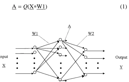
Multilayer feedforward networks have the capability of learning the internal representation of complex non-linear systems, which makes them desirable can-didates in problems associated with system model-ling and control. Cybenko [12] proved that multi-layer perceptrons with only one hidden multi-layer and sigmoidal hidden layer activation are capable of approximating any continuous function to within an arbitrary accuracy. Therefore, three-layer neural networks are generally considered and studied in most of the published literature on training neural network algorithms. It should be noted that a gener-alisation of the algorithm to networks with more than one hidden layer is a straightforward extension. Before proceeding to describe the training algorithm, it is necessary to give an explicit description of a three-layer feedforward neural network. The archi-tecture of such a network is shown in Fig. 1, where X and Y are the input and output of the network, respectively. The network may be represented in block diagram form as a series of affine transform-ations W1 and W2, and a diagonal non-linear oper-ator Q with identical sigmoidal activations. In other words, each layer of the network is regarded as the composition of an affine transformation with a non-linear mapping:

A=Q(XⴱW1) (1)

Fig. 1. Architecture of a three-layer neural network.

Y=Q(AⴱW2) (2)

As observed, a three-layer neural network is denoted by f(W1,W2), where W1 and W2 are the weights of the connection. A is the output of the hidden layer in the network.

Here, let the input training data set X be a N×m

matrix; m is the number of input neurons and N is the length of the training data set. Similarly, the target data set T is an N×n matrix; n is the number

of output neurons. In practice, the number of input nodes and the number of neurons in the output layer are fixed by the number of inputs and outputs of the system being considered. However, the numbers and states of the neurons in the hidden layer are important design parameters: they not only deter-mine the structure of the network, but also play an important role in the approximation of the network. Unfortunately, all of the known algorithms and methods of training and constructing neural networks focus on the input-output training pairs, and the number of the neurons in the hidden layer. Few researchers have taken into consideration the state of the hidden layer neurons. In fact, the potential of the neuron states in the hidden layer can have a significant impact on the training process.

In this paper, we highlight the use of the hidden layer in the network after a brief review of the Least Square Backpropagation (LSB) method. In 1993, Konig and Barmann [8,9] separated neural networks into linear parts, summations of the weighted inputs to the neurons, and nonlinear parts, nonlinear activity functions (such as sigmoidal activation). While solving the linear parts optimally, they used the inverse of the activation to propagate the remaining error back into the previous layer of the neural networks. Therefore, the learning error is minimised on each layer separately from the output layer to the hidden and input layers by using the least squares method (see [8,9] for details). That is so-called Least Square Backpropagation. The con-vergence of the algorithm is much higher than that of the classical BP algorithm. However, the draw-back of the LSB algorithm is that the training error cannot be further reduced after the first two or three iterations.

on the objectives set out by the designer. Next, we consider how to adjust the output of the hidden layer and make it satisfy those requirements. Although there are many ways to achieve that, here we prefer to introduce the output as its input. The main reason is that it adds a feedback loop for each neuron. The neurons with feedback, as in a closed control system, can sense the changes in the output due to the process changes, and attempt to correct the output. The neurons without feedback lack this type of self-regulation [13].

Here we adjust both the outputs of the hidden layer and the weights of network. To achieve this target, the relationship between the outputs of the hidden layer and the outputs of the output layer should be predetermined, and a method to adjust the outputs of the hidden layer should be determ-ined. The overall training scheme is derived as fol-lows.

2.1. To Determine the Output R of Hidden Layer

Let us consider the above network. The structure of the network is m-p-n and is fully connected between layers. To obtain a good convergence, the first neu-ron in each layer is a bias node with a constant output of 0.5.

The weights on the connections between the input layer and the hidden layer form a matrix W1 of real numbers with elements wij(i=1,2,%m;

j=1,2,%p). An element w_ij connects the ith neuron

in the input layer with the jth neuron in the hidden layer. Row number 1 of W1 contains the weights of the initiating connections at the bias node of the input layer. Similarly, W2 is a p×n weight-matrix

between the hidden layer and the output layer. The neurons used in this paper are of a standard type. They first build a scalar product of the incoming signals with their respective weights. Afterwards, an activity function is applied, produc-ing the output of the neuron, which is sent to all neurons of the following layer or to the outside world, respectively. We use the standard sigmoid activation function with values between 0 and 1:

Q(x)=1/(1 + e−x) (3)

For a given N sets of input signals (each set contains

m real numbers between 0 and 1), there are N sets

of output values (each output set contains n real numbers between 0 and 1). We can summarise all given input signals in a matrix X with N rows and

m columns. Each row contains the signals of one

input set. All elements of the first column are

constant 0.5 (the outputs of the bias node of input layer). Similarly, we can summarise all output sig-nals we want to train the network in a matrix T with N rows and n columns (no bias column).

Propagating the given examples through the net-work, we get (by multiplying the input matrix with the weights matrix between the input layer and the hidden layer, applying the activation function to all matrix elements, and adding a bias constant column of 0.5):

A=[0.5兩Q(XⴱW1)] (4)

Y=Q(AⴱW2) (5)

where A and Y are the outputs of the hidden layer and output layer.

Teaching the network means trying to adjust the weights such that Y is equal to (or as close as possible to) T. By introducing

S=Q−1(T) (6)

let us reformulate the task of learning. Adjust the weights of the network such that S is as close as possible to AⴱW2. The problem of determining W2 optimally can be formulated as a linear least squares problem:

储AⴱW2−S储2 =minimal (7)

Note that, since Q is a nonlinear function, the minimum of Eq. (7) is not necessarily identical with the minimum of 储Y−T储2.

After obtaining an optimal set W2 of weights, we could determine a required output matrix R of the hidden layer, which is as close as possible to A, and fulfils

储RⴱW2−S储2=minimal (8)

Again, this is for a given matrix W2 and S, a linear least square problem. Equivalently, one can find the minimal norm solution of ⌬R in

储⌬RⴱW2−(S−AⴱW2)储2 =minimal (9)

and determine R as R=A+⌬R

Since the output of the bias node is a constant 0.5, we require the first column of ⌬R to vanish.

Hence, we have to reformulate Eq. (9) to take care of this constraint. Let T1 and ⌬T1 be the matrixes containing all columns of R and ⌬R, except for the

first, and V be the matrix containing all rows of W2 except for the first. We then have to solve the linear least squares problem.

储⌬T1ⴱV−(S−AⴱW2)储2=minimal (10)

Now the output R of the hidden layer has been determined.

Since the activation function (5) can only produce values between 0 and 1, this is only feasible if all elements of R are in this range. To transform R to a matrix with elements between 0 and 1, we con-struct a matrix C with p rows and columns such that

Rtrans=RⴱC−1 and Wtrans=CⴱW2 (12)

The minimal condition (10) is then still valid for the new matrices. Using the following notation:

␣k=

冘

␥_j,k

冒

N, k=1,2,%p (13)

␤k= max j=1,%,N

␥j,k, k=1,%p (14)

␥k= min j=1,%,N

␥j,k, k=1,%p (15)

we can define the elements of C:

c0,0=1, c0,k=2(␣k−max(0.5,␤k−␣k,

␣k−␥k)), k=1,%,p (16)

ck,k=2 max(0.5,␤k−␣k,␣k−␥k),

k=1,%,p (17)

All other elements of C are zeros. The inverse matrix of C has the same structure as C, with elements

c(−1)0,k = −c0,k/ck,k, k=1,%,p (18)

c(−1)k,k =1/ck,k, k=0,%,p (19)

With this choice of C, all elements of Rtrans are

between 0 and 1, and the average output of each node is 0.5. We can now use the formalism as (6) and (7) to teach the hidden layers of the networks to produce Rtrans. Therefore, the desired output of

the hidden layer is R=Rtrans.

2.2. Adjustment of Hidden Layer Output

The hidden layer is adjusted by adding the desired output of the hidden layer as the inputs. That is, the input of the hidden layer is not only the input samples, but also the desired output of the hidden layer calculated from the output of the network. Let the input weights of the hidden layer be Wr. Wr is a (m+p)×p matrix including the weights W1 from

input layer and the weights W for the added inputs– desired outputs of the hidden layer. Similarly, the input matrix Xr should be a N×(m+p) matrix. It

includes the sample inputs X and the added inputs R. Therefore,

Wr=[W1 W]T_{, Xr}=_{[X R] (20)}

XrⴱWr=Q−1(R) (21)

where Q−1(R) is the inverse function of sigmoid activation function.

To adjust the weights and make it equal to (or as close as possible to) Q−1(R), minimise

储Q−1(R)−XrⴱWr储. It becomes a least square prob-lem again, and can be solved as above. The solution of the least squares problem is the new weights for the hidden layer.

2.3. Description of the Complete Algorithm

To simplify the computation, the above process is improved slightly. The desired outputs of the hidden layer are initially set to zeros. The dimension of the weights remains unchanged during the overall training process.

The complete training procedure can be stated as follows:

1. Initialisation:

쐌 Set randomly initial values, between [−1, 1] for weights W1, W2 and set the desired output R of the hidden layer to zero. Form the input matrix Xr of hidden layer

2. Optimisation of the output layer weights:

쐌 Propagate the given input matrix Xr through the network and get the outputs of the hidden layer and the output layer.

쐌 Get the ‘desired’ weighted sums of the output neurons by inverse activation function Eq. (6).

쐌 Compute the optimal weights of output layer according to Eq. (7).

쐌 Determine the ‘required’ output of the hidden layer using Eqs (8) and (9).

쐌 Normalise the ‘desired’ output of the hidden layer through Eqs (13–19).

3. Optimisation of the hidden layer weights:

쐌 Determine the ‘desired’ weighted sum of the hidden neurons according to the desired output of the hidden layer computed from above step using Eq. (6).

쐌 Form the input matrix Xr of the hidden layer.

쐌 Compute the optimal weights Wr of the hidden layer using Eq. (7).

4. Repeat steps 2–3 until a certain error tolerance is satisfied.

Although the training process cannot be completed in one iteration because the desired output of the hidden layer is different every time, it can converge within three iterations in general.

is a nonlinear one, the linear minimum weighted sum error is not necessarily identical to the output error. Let the actual error and the weighted sum error be as follows:

E=

冘

i=1

冘

j=1

(Yij−Tij) (22)

Esum=

冘

i=1

冘

j=1

(Q−1(Yij)−Q−1(Tij)) (23)

Here, n is the number of neurons in the output layer and N is the length of the training set. In addition, the optimal weights for a neural network are not unique; there may be numerous optimal sets of weights.

The algorithm derived above is constructed for generality. The activity function can be adjusted to other ones according to the application. For example, the activation in the output layer can be set to a linear function. During numerical simulation, it is found that sometimes the training error for a network using a linear function in the output layer is unstable. This problem can be solved by adding a hidden layer to the networks. Then the training results are in harmony with those using a sigmoidal function in the output layer. Therefore, the network can be applied to some common regression prob-lems.

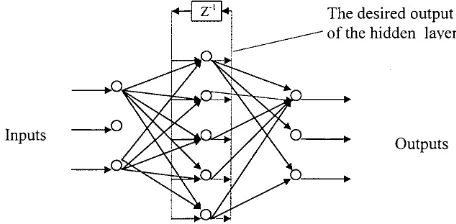
The proposed method is partially a recurrent neu-ral network, but different from conventional NNs. Conventional recurrent neural networks propagate back the outputs (or parts) of neurons in the hidden layer to their inputs through the recurrent paths, whereas the desired outputs of the hidden layer are used in this paper. It is a kind of teacher-forced training in the hidden layer so that a better training result can be achieved. Figure 2 shows the structure of the proposed network. The recurrent paths apply both during training and use. In the training process, since the network can reach its steady state in two feedforward propagations and the algorithm allows variation of the outputs, the networks can be trained

Fig. 2. Structure of the proposed network.

as general feedforward networks, although there is recurrency in it. It is not necessary to wait until the network reaches its steady state, as for recurrent networks. One advantage of the algorithm is being able to begin the training while the network is still in its dynamic period. During use, the network needs only two feedforward propagations to reach its steady states before a result is extracted, because the delay in the recurrent paths is very small.

3. Numerical Simulation Results

In this section, we present some numerical experi-mental results for the proposed algorithm. The efficiency of a training procedure depends mainly upon the training error and convergence speed.

To evaluate the performance of the training method presented, some comparisons with other methods have been carried out. We have im-plemented the following: the well-known classical BP algorithm, Quasi-Newton BFGS algorithm [14], Least square algorithm and the algorithm presented in this paper to train the networks with the same structure.

3.1. Case 1. MIMO Nonlinear System

Consider the nonlinear mapping of eight input quan-tities xi into three output quantities yi, defined by

y1 =(x1x2 + x3x4 + x5x6+ x7x8)/4

y2 =(x1+ x2+ x3+ x4+ x5+ x6

+ x7+ x8)/8

y3 =(1−y1)2 (24)

All three functions are defined for values between 0 and 1, and produce values in this range. For the training set, 100 sets of input signals xi were

gener-ated with a random number generator; the corre-sponding yi were computed using Eq. (24). The error

reported is the average absolute error on this learn-ing set example and output nodes:

⌬ =

冉

冘

冘

兩Yi,j−Ti,j兩

冊冒

The starting values for the weights of the networks have also been determined between 0 and 1 using a random number generator.

The errors for the BP algorithm are obtained after 2000 iterations. The errors for LSB, BFGS Quasi-Newton and the proposed algorithms are obtained after 10 iterations. The BP algorithm is the standard BP algorithm [1] with a learning rate of 0.1 and momentum factor of 0.9. One iteration (or epoch) indicates that all sets of input signals Xi are sent to

a certain network, a set of corresponding outputs of the network is obtained, and all the weights are adjusted once [15]. In fact, the LSB method and the algorithm presented need about twice the com-puter time of the backpropagation method per iter-ation, independent of the network’s structure [8].

Comparing the results in Table 1, the perform-ances of the proposed algorithm for the networks 8-12-3, 8-16-3, 8-24-3 and 8-36-3 are obviously the best ones. The training errors have been improved from 86.5% to 92.6% compared to the errors by using the LSB algorithm, and from 96.8% to 99.1% compared to the errors by using the BFGS Quasi-Newton algorithm.

The BFGS Quasi-Newton algorithm is generally faster than the conjugate gradient algorithms, but requires storage of the approximate Hessian matrix, and is slower than those algorithms developed from LSB. By comparison, it is found that the training errors of the method presented reduce iteratively, but the errors of the LSB don’t reduce after three iterations.

3.2. Case 2. Prediction of the Chaotic Mackey-Glass Time Series

Mackey and Glass modelled the chaotic oscillations in physiological processes. It is shown as

x(k + 1)−x(k)= 0.2x(k−␶)

1 + x10_(k−␶₎

−0.1x(k), ␶=17 (26) One thousand training samples were generated according to Eq. (26). The input vector of the net-work consists of past values of X, i.e., x(k), x(k−1),

Table 1. Training errors of the three methods.

Algorithm 8-12-3 8-16-3 8-24-3 8-36-3

BP 0.0218 0.0193 0.0174 0.0346

BFGS Quasi- 0.0751 0.0734 0.0705 0.0872

Newton

LSB 0.0178 0.0165 0.0218 0.0109

The Proposed 0.0024 0.0012 0.0009 0.0008

Method

x(k−2),%,x(k−16). The target is x(k+1). The

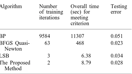
net-works retrained to predict the coming x(k+1) from the 17 past values. The first 750 samples are used as the training set; the rest are used to test the performance of the trained networks. The initial values of the weights of all the networks are gener-ated randomly between 0 and 1. The first 17 samples are initialised randomly between 0 and 1. All desired outputs are scaled between 0 and 1 through linear mapping. Table 2 shows the performance results compared with the BP, LSB and BFGS Quasi-Newton algorithms. The training error tolerance is chosen to be 0.02.

The overall time is the training time of each corresponding method for reaching the criterion, using Matlab to implement the simulations in an IBM586. As shown in Table 2, to reach the training error tolerance, 0.02, the proposed method takes a little longer than LSB, due to a greater network complexity. However, the testing error of the pro-posed method is less than that of LSB. By compari-son, the BFGs Quasi-Newton algorithm has the low-est tlow-esting error, but it needs 7 or 8 minutes, 50 times longer than that of the proposed algorithm to reach the same error tolerance. The Quasi-Newton BFGS algorithm still suffers from the typical handi-cap; slow convergence of all steepest descent approaches. The BP algorithm takes more than three hours to reach the same error tolerance, and the testing error is the largest one among the four methods.

3.3. Case 3. Comparison with General Recurrent Neural Networks

It may be argued that the improvements of the training algorithm may be due to the addition of the weights in the hidden layer. To demonstrate that the above is not true, we compare the performance

Table 2. Performance of different algorithms for Mackey-Glass series.

Algorithm Number Overall time Testing

of training (sec) for error

iterations meeting criterion

BP 9584 11307 0.051

BFGS Quasi- 63 468 0.023

Newton

LSB 3 6.38 0.034

The Proposed 2 8.79 0.028

Fig. 3. Performance of LSB for RNN, Quasi-Newton BFGS

algorithm and the proposed method for the MIMO case. ——: proposed method; ...: LSB for Recurrent Neural Networks; -.-.-.-: Quasi-Newton BFGS algorithm.

of the proposed algorithm with the LSB method for a recurrent neural network with the same topology (same number of neurons and same weights).

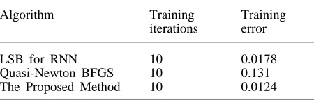
Take the MIMO case again, where 100 samples are applied. The converging performances are shown in Fig. 3. The training errors and iterations corre-sponding to the errors are shown in Table 3. As shown in Fig. 3, in the MIMO case, the errors of LSB for RNN and the proposed method are nearly the same at the first two iterations. Afterwards, the error of LSB for RNN has no further reduction; however, the error of the proposed scheme can be reduced gradually. The error for the Quasi-Newton BFGS method is much higher than the other two algorithms.

4. Conclusions

A new training algorithm for multilayer networks is proposed and tested, which optimises the network weights through an iterative process layer-by-layer. The proposed training algorithm takes the output of

Table 3. Training errors and number of iterations of LSB for RNN and the proposed method for the MIMO case.

Algorithm Training Training

iterations error

LSB for RNN 10 0.0178

Quasi-Newton BFGS 10 0.131

The Proposed Method 10 0.0124

nodes in the hidden layer into consideration. It not only adjusts the weights of the networks, but also adjusts the output of the hidden layer. To achieve the goal of adjusting the output of the hidden layer, a new structure for multi-layer neural networks is suggested. The proposed network works like a recur-rent neural network, but it can reach its steady state very quickly because of its novel training algorithm. From the simulation results, it is observed that after the first three epochs for LSB, no substantial progress could be achieved by continuing the iter-ations. However, for the proposed method, not only can it further reduce the error, but it can also converge within 10 iterations. In the case of the classical BP algorithm, to reach the same accuracy it will take nearly 1000 iterations [2,3]. Although the Quasi-Newton BFGS algorithm is the fastest algorithm among the conjugate gradient methods, it takes more than 50 times longer than that of the proposed algorithm to reach the same error tolerance for the same application. The Quasi-Newton BFGS algorithm still suffers from the typical handicap; slow convergence of all steepest descent approaches. All the simulation results presented show that the proposed algorithm is orders of magnitude faster than the classical backpropagation and Quasi-New-ton BFGS algorithms. The performance of the pro-posed method is also better than that of the original LSB method, with its inherent drawback that its training error cannot be reduced further after three iterations.

Acknowledgements. The first and second authors gratefully acknowledge the financial support of the Hong Kong Polytechnic University through the grant G-V067.

References

1. Rumelhart DE, Hinton GE, Williams RJ. Learning internal representations by error propagation in parallel distributed processing. In: DE Rumelhart, JL Mc-Clelland, eds., Explorations in the Microstructures of Cognition, Vol. 1. Foundations, MIT Press, Cam-bridge, MA, 1986; 318–362

2. Battiti R. Accelerating backpropagation learning, two optimisation methods. Complex System 1989; 3: 331–342

3. Yam YF, Chow TWS. Extended backpropagation algorithm. Electr Lett 1993; 29(9): 1701–1702 4. Humpert BK. Improving backpropagation with a new

error function. Neural Networks 1994; 7(8): 1191– 1192

6. Kinnebrock W. Accelerating the standard backpropag-ation method using genetic approach. Neurocomputing 1994; 13: 583–588

7. Zhang B, Zhang L, Wu F. Programming based learn-ing algorithms of neural networks with self-feedback connections. IEEE Trans Neural Networks 1995; 6(3): 771–778

8. Konig FB, Barmann F. A learning algorithm for multi-layered neural networks based on linear least square problems. Neural Networks 1993; 6: 127–131 9. Konig FB, Barmann F. On a class of efficient learning

algorithms for neural networks. Neural Networks 1992; 5: 139–144

10. Coetzee FM, Stonick VL. Topology and geometry of single hidden layer network least squares weight solutions. Neural Computation 1995; 7: 672–705

11. Ergezinger S, Thomsn E. An accelerated learning algorithm for multilayer perceptrons: Optimisation layer by layer. IEEE Trans Neural Networks 1995; 6(1): 31–42

12. Cybenko G. Approximation by superposition of a sigmoidal function. Math. Control Signals Syst 1989; 2: 303–314

13. Dorf RC, Bishop HR. Modern Control System. Addison-Wesley, 1995

14. Demuth H, Beale M. Neural network Toolbox for use with MATLAB. The Matlab Works, Inc., January 1998 pp 5-20–5-40