This is a repository copy of A classification of poromechanical interface elements.
White Rose Research Online URL for this paper:
http://eprints.whiterose.ac.uk/141940/
Version: Accepted Version
Article:
de Borst, R. orcid.org/0000-0002-3457-3574 (2017) A classification of poromechanical
interface elements. Journal of Modeling in Mechanics and Materials, 1 (1). 20160160.
ISSN 2328-2355
https://doi.org/10.1515/jmmm-2016-0160
© 2017 Walter De Gruyter GmbH. This is an author produced version of a paper
subsequently published in Journal of Modeling in Mechanics and Materials. Uploaded in
accordance with the publisher's self-archiving policy.
[email protected] Reuse
Items deposited in White Rose Research Online are protected by copyright, with all rights reserved unless indicated otherwise. They may be downloaded and/or printed for private study, or other acts as permitted by national copyright laws. The publisher or other rights holders may allow further reproduction and re-use of the full text version. This is indicated by the licence information on the White Rose Research Online record for the item.
Takedown
If you consider content in White Rose Research Online to be in breach of UK law, please notify us by
A classification of poromechanical interface elements
Ren´e de Borsta,∗
aUniversity of Sheffield, Department of Civil and Structural Engineering, Sir Frederick Mappin Building, Mappin Street, Sheffield S1 3JD, UK
Abstract
Interface elements are a classical approach to represent discrete cracks, joints and faults. The basic kinematic and constitutive aspects are recapitulated and the extension to hydromechanical conditions is elaborated. A classification is presented of hydrome-chanical interface elements, depending on the multiplicity of the pressure degree of freedom, and the physical implications of the different possibilities are explained.
Keywords: poromechanics, fracture, hygro-mechanical interfaces, finite elements
1. Introduction
Fracture in fluid-saturated porous media is a challenging, multi-scale problem with moving internal boundaries, characterised by a high degree of complexity. Moreover, fracture initiation and propagation in fluid-saturated porous materials occur frequently, indicating that there is also a large practical relevance. The existence and propagation of cracks in porous materials can be undesirable, like those that form in human tissues, or when the storage of waste in rocks or salt domes is concerned. But cracking can also be a pivotal element in an industrial process, for example hydraulic fracturing in the oil and gas industry. Another important application area is the rupture of geological faults, where the change in geometry of a fault can drastically affect local fluid flow as the faults can act as channels in which the fluid can flow freely.
Interface elements are a powerful and relatively simple manner to simulate crack initiation and propagation [1, 2]). Remeshing has been introduced to decouple the crack propagation path from the original mesh [3, 4, 5, 6, 7]. The extended finite element method [8, 9] has been proposed as an alternative approach. It decouples the crack propagation path from the underlying discretisation, and has been a main carrier of numerical approaches to fracture for more than a decade. The extension to fracture in fluid-saturated porous media has been accomplished as well [10, 11, 12, 13, 14, 15, 16]. The main subject of this paper is a classification of discretisation technologies for poroelastic interfaces, starting from the case that the pressure is continuous across the discontinuity, but where the pressure gradient is discontinuous. This relatively simple formulation already allows for the transport and storage of liquid inside the crack,
∗Corresponding author: Ren´e de Borst
provided that the pressure gradient can be discontinuous. In the extended finite element method this is achieved by partitioning the pressures at both sides of the discontinuity by a signed distance function [11, 13]. In interface elements [17] a discontinuous pressure gradient across the discontinuity comes in naturally, as by definition they are
C0-continuous with respect to the pressure across the interface. Pressure continuity has also been assumed by Armero and Callari [18] using a discontinuous enrichment for the displacements exploiting the Enhanced Assumed Strain concept. In the latter case flow and storage inside the cracks is not enabled since, within the element, the continuity of the pressure field is higher thanC0.
Other poroelastic interfaces can be constructed starting from the assumption that the pressure is discontinuous orthogonal to the discontinuity [10, 12, 19, 20], or that a Dirac function is superimposed on the interpolation functions for the pressure field as in [21]. Again, it depends on the applied discretisation technology whether flow and storage are enabled inside the crack. In [10, 12] this has been achieved by partition-ing the pressure field at both sides of the discontinuity through a Heaviside function placed at it, which enables the gradient to be discontinuous as well. Likewise, it is naturally embedded in interface elements with a double pressure node because of the
C−1 continuity in the pressure field at the interface [19, 20]. It is finally noted that
(pressure-continuous) poroelastic interface elements have also been developed within the context of isogeometric analysis [22], including the possibility of fluid flow and storage in the discontinuity [23].
Herein, we start with a brief recapitulation of three-dimensional, mechanical inter-face elements. Next, extension is made to interinter-faces that are embedded in a poromechi-cal medium, and that allow for mass transport within the interface. Three formulations are distinguished, with a single pressure node, a double pressure node, and a triple pressure node at the discontinuity. The strong and weak forms are given, as well as the discretised format, and the physical implications of the different choices. Examples with single and double pressure nodes conclude the paper.
2. Standard interface elements
Interface elements are normally inserted a priori in the finite element mesh, unless remeshing is used. For stationary discontinuities, or when the direction of the prop-agation is known, interface elements can be used in a simple manner. When internal discontinuities propagate, they can be used in combination with remeshing.
The kinematic quantities in continuous interface elements are a set of mutually orthogonal, relative displacements:~unfor the opening mode, and~us,~utfor the
two sliding modes. When collecting the relative displacements in a vector
~u=(~un,~us,~ut)T, (1)
which is defined in a local s,n,t-coordinate system, they can be related to the
displace-ments u+at the upper side of the interface,Γ+d, and the displacements u−at the lower side of the interface,Γ−d, via
s n
Γ nΓd
d
h s
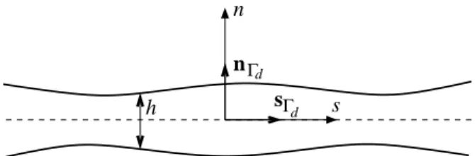
Figure 1: Geometry and local coordinate system in the interface
where u+,u−are expressed in the global x,y,z-coordinate system, and R=(sΓ
d,nΓd,tΓd)
is the standard rotation matrix between the local and the global coordinate system, with
sΓd,tΓdmutually orthogonal unit vectors aligned with the discontinuity, and nΓdthe unit vector normal to the discontinuity, see also Figure 1 for a two-dimensional representa-tion. The displacements are interpolated in a standard manner as:
u=Ha, (3)
where
H=
h 0 0
0 h 0
0 0 h
(4)
and a is the nodal displacement array that contains the degrees of freedom related to the
N nodes in case of a standard continuum element. For an interface element, however,
the nodes are doubled, one set of N nodes for theΓ+
d side of the interface, and another
set of N nodes for theΓ− side, cf Figure 2. The 1×N matrices h contain the shape functions h1, ...,hN:
h=
h1
... ...
hN
. (5)
The relation between the nodal displacements and the relative displacements for inter-face elements then reads:
~u=R u+−u−=R Ha+−Ha−=RBd˜a, (6)
with
Bd=
−h +h 0 0 0 0
0 0 −h +h 0 0
0 0 0 0 −h +h
. (7)
the relative displacement-nodal displacement matrix for the interface element, and ˜a containing the discrete nodal displacements at both sides of the interface expressed in the global x,y,z-coordinate system. It is noted that, although ˜a contains twice the
(a) (b)
pressure node displacement node
(c)
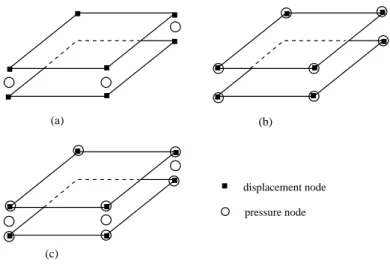
Figure 2: Interface elements enriched with pressure nodes
In the local coordinate system, the cohesive tractions tloc
d are related to the relative
displacements~uvia a nonlinear relation:
tlocd =tlocd (~u, κ), (8)
withκa history parameter. Similar to the relative displacements, the traction vector tloc d
can be related to the tractions in the global coordinate system using the rotation matrix
R:
tlocd =Rtd (9)
For use in a Newton-Raphson iterative procedure this constitutive relation can be lin-earised as:
dtlocd =Ddd~u, (10)
with ’d’ a small increment, and
Dd=
∂tlocd
∂~u. (11)
The limiting case that tloc
d =0 obviously represents a traction-free crack.
For the purely mechanical case, the equilibrium equation reads:
∇ ·σσσ=0. (12)
After multiplication by a test functionηηηand application of Gauss’ theorem, the weak form is obtained:
Z
Ω
∇ηηη:σσσdΩ
− Z
Γ+
d
η ηη+·(nΓ+
d ·σσσ
+)dΩ−
Z
Γ− d
ηηη−·(nΓ−
d ·σσσ
−)dΩ =
Z
Γt
η η η·tpdΩ,
Γ Γ
d _ +
d
n
n
Γ Γ
d
_
d Γ+
nΓ tp
up
q q
qd_
+
d Ω
p p
p
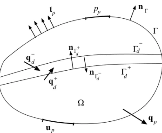
Figure 3: BodyΩwith external boundaryΓand internal boundariesΓ+
dandΓ
−
d
with tpthe prescribed tractions at the external traction boundaryΓt. SinceΓd = Γ+d =
Γ−d, which defines the zero-thickness interfaceΓd, the surface integrals at this interface
can be elaborated as follows. We define:
nΓd=nΓ−d =−nΓ+d (14)
see also Figure 3. Next, we assume traction continuity between the interface and the bulk:
σ σ σ+·nΓ−
d =−σσσ
−·n Γ+
d =td, (15)
with td the cohesive tractions. Using Equation (15), the equilibrium equation,
Equa-tion (13), can be reworked as:
Z
Ω
∇ηηη:σσσdΩ +
Z
Γd
~ηηη·tlocd dΓ =
Z
Γt
η
ηη·tpdΓ, (16)
We discretise the test functionηηηin a Bubnov-Galerkin sense:
η
ηη=Hw (17)
with w a nodal array. Noting that
~ηηη=RBdw˜ (18)
cf. Equation (6), and following standard procedures the discrete form of Equation (16)
results: Z
Ω
wTBTuσσσdΩ +
Z
Γd
˜
wTBTdRTtlocd |{z}
td dΓ =
Z
Γt
wTBTutpdΓ, (19)
with
L= ∂
∂x 0 0
0 ∂∂y 0
0 0 ∂∂z
∂ ∂y
∂ ∂x 0
0 ∂∂z ∂∂y
∂ ∂z 0
∂ ∂x (21)
the matrix that relates the strains,ǫǫǫ, to the displacements a continuum element: ǫǫǫ =
Lu. Considering that this identity must hold for all admissible test functions, and
rearranging yields:
fext−fint=0. (22)
with the external force vector
fext=
Z
Γt
BTutpdΓ (23)
and the internal force vector
fint=
Z
Ω
BTuσσσdΩ +
Z
Γd
BTdtddΓ. (24)
The set of Equations (22) is generally nonlinear and is typically solved using a Newton-Raphson scheme for every time step. Defining the material tangential stiffness matrix
Dj−1=
∂σσσ ∂ǫǫǫ
j−1, (25)
which sets the relation between the change in the stress dσσσand that in the strain, dǫǫǫ, from iteration j−1 to iteration j in the continuum, cf. [24]:
dσσσ=Dj−1dǫǫǫ, (26)
and utilising the material tangential stiffness matrix for the interface, Dd, the tangential
stiffness matrix after iteration j−1, can be derived as:
Kj−1=
∂fint j−1
∂a = Z
Ω
BTuDj−1BudΓ
| {z }
KΩ
j−1
+
Z
Γd
BTdRTDd,j−1RBddΓ
| {z }
KΓd
j−1
. (27)
The iterative improvement da of the nodal displacements in iteration j then follows from:
Kj−1da=fext−fintj−1. (28)
Interface elements are often inserted in the finite element mesh prior to the compu-tation, and a finite stiffness must be assigned in the pre-cracking phase with at least the diagonal elements being non-zero. Prior to crack initiation, the stiffness matrix in the interface element reads:
Dd=
dn 0 0
0 ds 0
0 0 dt
with dn a high (dummy) stiffness normal to the interface and ds and dt the
tangen-tial stiffnesses. It is noted that in the pre-cracking phase the numerical integration of interface elements can entail inaccuracies [2].
3. Poromechanical interface elements
For a poromechanical interface element, each node is augmented with one or more pressure degrees of freedom. For a single pressure degree of freedom, the pressure is continuous at the internal discontinuity [11, 13, 17, 23]. When two pressure degrees of freedom are added, the pressure can be discontinuous across the internal boundary Γd[10, 12, 19, 20]. Alternatively, one can assume that the same pressure exists at both
sides of the discontinuity, but that this pressure is different from that inside the discon-tinuity [21]. This model, in which a regularised Dirac function is superimposed on the regular pressure field, also requires two degrees of freedom at the internal boundary. However, from a physical point of view the case that the pressure is the same at both sides of the interface may be less relevant, and its treatment is not pursued here. The most general case is when the pressures at both sides of the crack are allowed to differ, and can be different from the fluid pressure within the crack as well, a model with three pressure nodes ensues [26]. It is finally noted that all three options result in a pressure gradient which can be discontinuous, allowing for storage and fluid flow within the discontinuity. Indeed, the pressure across the interface element is at most interpolated with aC0-continuity, yielding a pressure gradient that is at mostC−1-continuous.
In a fluid-saturated porous medium, the total stress is composed of a solid and a fluid part:
σ σ
σ=σσσs+σσσf (29)
Using the Biot coefficientα, which takes into account the compressibility of the solid grains [27], the total stress can be written as:
σσσ=σσσs−αpI (30)
with p the (apparent) fluid pressure and I the unit tensor. In a similar spirit we have
σσσ+·nΓ−
d =−σσσ
−·n Γ+
d =td−pnΓd (31)
instead of Equation (15). When inserting Equations (30) and (31) into the weak form of the equilibrium equation, Equation (13), and using Equation (14), we now obtain:
Z
Ω
∇ηηη: (σσσs−αpI)dΩ +
Z
Γd
~ηηη·(tlocd −pnlocΓ
d) dΓ =
Z
Γt
η η
η·tpdΓ. (32)
The mass balance of a fluid-saturated porous medium reads, e.g. [10, 27]:
α∇ ·˙us+nf ( ˙uf −˙us)+
1
M
∂p
∂t =0 (33)
with nf the porosity and M the Biot modulus. Inserting Darcy’s relation
with kf the permeability then gives:
α∇ ·˙us− ∇ ·
kf∇p
+ 1
M
∂p
∂t =0. (35)
To arrive at the weak form, we multiply by a test function for the pressure,ζ. Integrat-ing over the domainΩand using the divergence theorem and the appropriate boundary condition leads to:
− Z
Ω
αζ∇ ·˙usdΩ−
Z
Ω
kf∇ζ· ∇p dΩ−
Z
Ω
ζ 1
M
∂p
∂tdΩ
− Z
Γ+
d
ζ+nΓ+
d ·q
+
ddΓ−
Z
Γ− d
ζ−nΓ−
d ·q
−
ddΓ =
Z
Γq
ζnΓ·qpdΓ,
(36)
with qpthe prescribed flux on the flux boundaryΓq. It is noted that the equation has
been multiplied by -1 as well in order to preserve symmetry after linearisation. Having assumed equilibrium between the cavity and the bulk, Equation (15), in-voking Equation (14), and noting that the (cohesive) tractions td have a unique value,
the fluid pressure p has the same value at both faces of the cavity: p=p+=p−. Using a Bubnov-Galerkin approach, this implies that also the test functionζattains the same value at both faces: ζ = ζ+ = ζ−. With this corollary, the weak form of the mass balance is modified as:
− Z
Ω
αζ∇ · ˙usdΩ−
Z
Ω
kf∇ζ· ∇p dΩ−
Z
Ω
ζ 1
M
∂p
∂tdΩ
+
Z
Γd
ζnΓd·~qddΓ =
Z
Γ
ζnΓ·qpdΓ
(37)
A jump in the flux,
~qd=q+d −q−d (38)
has now emerged in the integral for the discontinuity, see Figure 3. This term is mul-tiplied by the normal nΓd toΓd, resulting in a jump of the flow normal to the internal discontinuity. Accordingly, the flow can be discontinuous atΓd and some of the fluid
that flows into the crack can be stored or be transported within the crack. The jump in the flux is therefore a measure of the net fluid exchange between a discontinuity (the cavity) and the surrounding bulk material. It is emphasised that because of the pres-ence of a discontinuity inside the domainΩ, the power of the external tractions onΓd
and the normal fluid flux through the faces of the discontinuity are essential features of the weak formulation. Indeed, these terms enable the momentum and mass couplings between a discontinuity – the mesoscopic scale – and the surrounding porous medium – the macroscopic scale.
3.1. Interface elements with a continuous pressure
We first consider the case of a continuous pressure across the interface element, so that there is a single pressure node only, Figure 2(a). The pressure in the interface is then interpolated as:
where
hTp =(hp)1, ...,(hp)N
(40) contains the interpolation polynomials (hp)1, ...,(hp)Nfor the pressure, and
p= p1 ... ... pN (41)
contains the nodal values of the pressure p. We discretise the test functionζ for the pressure also in a Bubnov-Galerkin sense:
ζ=hTpz, (42)
with z the corresponding nodal array. The gradients needed in subsequent elaborations are assembled in a matrix
Bp=
∂(hp)1
∂x ... ...
∂(hp)N
∂x
∂(hp)1
∂y ... ...
∂(hp)N
∂y
∂(hp)1
∂z ... ...
∂(hp)N
∂z (43) so that
∇p=Bpp. (44)
When we define the external force vector fextas in Equation (23),
fuext=
Z
Γt
BTutpdΓ (45)
formally the same format for the discrete equilibrium equation is obtained as in Equa-tion (22):
fuext−fuint=0. (46)
However, the interface term is now elaborated as:
Z
Γd
~ηηη·(tlocd −pnlocΓ
d) dΓ =
Z
Γd
˜
wTBTd(td−pnΓd) dΓ, (47) so that the internal force vector reads:
fuint=
Z
Ω
BTu(σσσs−αpm)dΩ +
Z
Γd
BTd(td−pnΓd) dΓ. (48)
fint
u then results in:
Kuu,j−1=
∂fuint,j−1
∂a = Z
Ω
BTuDj−1BudΩ
| {z }
KΩ
uu,j−1
+
Z
Γd
BTdRTDd,j−1RBddΓ
| {z }
KΓd
uu,j−1
(49a)
Kup,j−1=
∂fuint,j−1
∂p =− Z
Ω
αBTumhTpdΩ
| {z }
−KΩ
up,j−1
− Z
Γd
BTdnΓdh
T pdΓ
| {z }
−KΓd
up,j−1
. (49b)
We next recall the weak form of the mass balance, Equation (37):
− Z
Ω
αζ∇ ·˙usdΩ−
Z
Ω
kf∇ζ· ∇p dΩ−
Z
Ω 1
Mζ˙pdΩ
+
Z
Γd
ζnΓd·~qddΓ =
Z
Γ
ζnΓ·qpdΓ.
Substituting the discretisations for the displacement field usand the pressure field p
along with that for the corresponding test functionsζ, and requiring that the result holds for all admissible test functions, leads to the discrete format:
− Z
Ω
αhpmTBudΩ
! ˙a−
Z
Ω
kfBTpBpdΩ
!
p−
Z
Ω 1
Mhph
T pdΩ
! ˙p
+
Z
Γd
hpnTΓd~qddΓ
| {z }
QΓd
=
Z
Γ
hpnTΓqpdΓ. (50)
where QΓdrepresents the rate of fluid exchange between the cavity and the bulk. The integration over a time step∆t is commonly carried out using a Backward Euler
scheme:
˙ (•)=(•)
t+∆t−(•)t
∆t (51)
with the superscript denoting at which time the quantity is evaluated. Substitution of the time integration scheme into Equation (50) yields, after multiplication by∆t in
order to preserve a symmetric tangential stiffness matrix:
fintp =fpext (52)
with the external force vector:
fextp = ∆t
Z
Γ
and the internal force vector:
fintp =−
Z
Ω
αhpmTBudΩ
!
| {z }
−KΩ
pu,j−1=−
KΩ
up,j−1
T
ut+∆t− Z
Ω 1
Mhph
T pdΩ
!
| {z }
−KΩ(1)pp,j−1
pt+∆t− ∆t
Z
Ω
kfBTpBpdΩ
!
| {z }
−KΩ(2)pp,j−1
pt+∆t
+
Z
Ω
αhpmTBudΩ
!
| {z }
−KΩ
pu,j−1=
KΩ
up,j−1
T
ut+
Z
Ω 1
Mhph
T pdΩ
!
| {z }
−KΩ(1)pp,j−1
pt+ ∆tQΓd.
(54) The contributions to the tangential stiffness matrix follow in the usual manner, by differentiating fint
p with respect to a and p, respectively:
∂fint p,j−1
∂a =K
Ω
pu,j−1+ ∆t
∂QΓd
∂a (55a)
∂fint p,j−1
∂p =K
Ω(1) pp,j−1+K
Ω(2) pp,j−1+ ∆t
∂QΓd
∂p . (55b)
Hence, the complete linearised set of equations, needed in a Newton-Raphson frame-work, reads: KΩ
uu,j−1+K
Γd
uu,j−1 K
Ω
up,j−1+K
Γd
up,j−1
KΩpu,j−1+ ∆t ∂QΓd
∂a
j−1 K
Ω(1) pp,j−1+K
Ω(2) pp,j−1+ ∆t
∂QΓd ∂p
j−1
da dp = fext u
fextp
− fint u,j−1
fint p,j−1
. (56) It is noted that the terms KΓd
up and∆t
∂QΓd
∂a render the tangential stiffness matrix non-symmetric, and are omitted in most computations.
To compute
QΓd =
Z
Γd
hpnTΓd~qddΓ (57)
we recall that the local rate of fluid exchange between an open cavity and the surround-ing bulk material is given by [11, 13]:
nTΓ
d~qd=nf
h3
12µ ∂2p
∂s2 +
h2
4µ ∂h
∂s
∂p
∂s −h
∂( ˙us)s
∂s − kf
nf
∂2p
∂s2
! −∂h
∂t
!
(58)
where the resemblance to Reynolds lubrication equation can be noted [28], andµis the fluid viscosity and h the width of the cavity, Figure 1. From this equation we observe that higher-order derivatives and non-standard terms have to be computed. Therefore, the matrix
B2p=
∂2(h
p)1
∂x2 ... ... ∂(hp)N
∂x2
∂2(h
p)1
∂y2 ... ... ∂(hp)N
∂y2
∂2(h
p)1
∂z2 ... ... ∂(hp)N
∂z2
is defined such that
∂2p
∂s2 =s T
ΓdB
2
pp, (60)
the matrix
Bd,s=
−∂∂hs +∂∂hs 0 0 0 0
0 0 −∂h
∂s +
∂h
∂s 0 0
0 0 0 0 −∂∂hs +∂∂hs
, (61)
which is needed to compute
∂h
∂s =n
T
ΓdBd,sa, (62)
while the tangential gradient of the solid velocity can be approximated as the average of the velocities atΓ+
d andΓ
−
d:
∂( ˙us)s
∂s ≈s
T
Γd
¯
Bd,s˙a, (63)
The operator matrix ¯Bd,s is built similar to Bd,s, except that the coefficients±1 are
replaced by12. Using these identities, we obtain
QΓd =
Z
Γd
hp
nf
12µ
nTΓ
dBda
3 sTΓ
dB
2 pp
+nf 4µ
nTΓ
dBda
2 nTΓ
dBd,sa s
T
ΓdBpp
−nTΓ
dBda
sTΓ
d
¯ Bd,s˙a−
kf
nf
sTΓ
dB
2 pp
! −nTΓ
dBd˙a
!
dΓ.
(64)
From this expression it is evident that the derivatives
∂QΓd
∂a and
∂QΓd
∂p (65)
lead to very cumbersome and lengthy expressions, which is another reason why they are normally not incorporated in the tangential stiffness matrix. Moreover, ∂QΓd
∂p adds another non-symmetry to the tangential stiffness matrix.
3.2. Interface elements with a discontinuous pressure
In case of a possible discontinuous pressure across the interface element, i.e. when there are two pressure nodes, Figure 2(b), the fluid flux in the interface reads:
nΓd·~qd=−knd(p
+−p−)=−k
nd~p (66)
The discretisation of the pressure jump is similar to that of the displacement jump, cf. Equation (6),
~p=(p+−p−)=(hTpp+−hTpp−)=Hp˜p, (67)
with
Hp=
h
The array ˜p contains the discrete nodal pressures at both sides of the interface. Similar to the displacements, globally no degrees of freedom are added although ˜p contains twice the number of degrees of freedom as does p per element. Substitution of Equa-tion (68) into EquaEqua-tion (67) then gives:
nΓd·~qd=−kndHpp. (69)
An anomaly of the approach is that there is no (separate) pressure within the in-terface. As a consequence, the pressure vanishes from the stress continuity condition across the interface and, instead of Equation (48), we have for the interface contribution to the internal force vector:
fuint=
Z
Ω
BTu(σσσs−αpm)dΩ +
Z
Γd
BTdtddΓ. (70)
Since in the absence of an explicitly defined pressure in the discontinuity, fint
u no longer
depends on it, the interface stiffness term KΓd
up cancels as well, and only the interface
stiffness KΓd
uuremains.
The interface term in the mass balance also simplifies. Noting that, similar to the displacement discontinuity, the jump in the test function,~ζ, is interpolated in a Bubnov-Galerkin sense as:
~ζ=Hp˜z, (71)
the interface term in the weak form of the mass balance, Equation (37), can be
elabo-rated as: Z
Γd
~ζnΓd·~qddΓ =−˜z
T
Z
Γd
kndHTpHp˜pdΓ (72)
where Equation (69) has been used. Since this expression must hold for all admissible test functions for the pressure, the contribution that stems from the internal discon-tinuity to the internal force vector becomes, after multiplication by∆t for symmetry
reasons:
−∆t
Z
Γd
kndHTpHpdΓ
!
p (73)
Hence, the only non-vanishing contribution from the internal discontinuity to the tan-gential stiffness matrix becomes:
KΓd
pp=−∆t
Z
Γd
kndHTpHpdΓ. (74)
3.3. An independent pressure in the interface
The deficiency of the discontinuous pressure model can be remedied by superim-posing a (regularised) Dirac function for the pressure, in the spirit of the local enrich-ment proposed by [21]. The independent pressures are now p−at theΓ−d-side of the interfaceΓd, p+at theΓ+d-side and pd within the interface. Clearly, the existence of
an independent pressure within the discontinuity allows for modelling pressurising the crack, which permits extension of the modelling capabilities to hydraulic fracturing.
Different from the previous two cases, an explicit distinction must now be made between the inflow of fluid through theΓ−andΓ+-interfaces. In principle, the resistance at both boundaries can be different, and (time-dependent) expressions for leak-offhave been derived based on a heat conduction analogy [26]. Herein, we simply assume that the resistance to flow is the same at both boundaries of the cavity, knd. Then, the
following relation ensues between the flux into the discontinuity and the different fluid pressures:
nΓd·~qd=−knd(p −−p
d)−knd(p+−pd)=knd(2pd−p+−p−). (75)
The sum of the pressures p−and p+is interpolated as
p++p−=Hp˜p, (76)
with Hpredefined as
Hp=
h hTp h
T p
i
. (77)
Evidently, there must now be a separate interpolation for pd:
pd=hTdpd (78)
where the vector
hTd =((hd)1, ...,(hd)N) (79)
contains the interpolation polynomials for the pressure in the discontinuity, and
pd =
(pd)1
... ...
(pd)N
(80)
contains the nodal values of the pressure pd. We discretise the test functionζdfor the
pressure in the discontinuity also in a Bubnov-Galerkin sense:
ζd =hTdzd, (81)
with zdthe corresponding nodal array. Again, gradients are needed and are assembled
in a matrix:
Bpd=
∂(hd)1
∂x ... ...
∂(hd)N
∂x
∂(hd)1
∂y ... ...
∂(hd)N
∂y
∂(hd)1
∂z ... ...
∂(hd)N
∂z
so that
∇pd =Bpdpd (83)
Using Equations (76) and (78), Equation (75) can be rewritten as:
nΓd·~qd=2kndh
T
dpd−kndHp˜p. (84)
Since there is now an independent pressure pdwithin the discontinuity, the internal
force vector that stems from the momentum balance remains as in the single pressure model:
fuint=
Z
Ω
BTu(σσσs−αpm)dΩ +
Z
Γd
BTd(td−pdnΓd) dΓ, (85) cf. Equation (48). Three separate contributions to the tangential stiffness matrix can now identified:
Kuu,j−1=
∂fuint,j−1
∂a = Z
Ω
BTuDj−1BudΩ
| {z }
KΩ
uu,j−1
+
Z
Γd
BTdRTDd,j−1RBddΓ
| {z }
KΓd
uu,j−1
(86a)
Kup,j−1=
∂fuint,j−1
∂p =− Z
Ω
αBTumhTpdΩ
| {z }
−KΩ
up,j−1
(86b)
Kud,j−1=
∂fuint,j−1
∂pd
=− Z
Γd
BTdnΓdh
T ddΓ
| {z }
−KΓd
ud,j−1
. (86c)
After multiplication by∆t for symmetry-preserving reasons, the contributions from
the global mass balance to the tangential stiffness become:
Kpu,j−1=
∂fintp,j−1
∂a =− Z
Ω
αhpmTBu
| {z }
−KΩ
pu,j−1
(87a)
Kpp,j−1=
∂fintp,j−1
∂p =− Z
Ω 1
Mh
T phpdΩ
| {z }
−KΩ(1)pp,j−1
−∆t
Z
Ω
kfBTpBpdΩ
| {z }
−KΩ(2)pp,j−1
−∆t
Z
Γd
kndHTpHpdΓ
| {z }
−KΓd
pp,j−1
(87b)
Kpd,j−1=
∂fintp,j−1
∂pd
=2∆t
Z
Γd
kndhphTddΓ
| {z }
KΓd
pd,j−1
. (87c)
where the weak form of Equation (84) has been exploited:
Z
Γd
ζnΓd·~qddΓ =
Z
Γd
2kndζhTdpddΓ−
Z
Γd
To complete the set of governing equations, the local mass balance at the disconti-nuity
2kndpd−knd(p−+p+)−nf
h3
12µ ∂2p
d
∂s2 +
h2
4µ ∂h
∂s
∂pd
∂s −h
∂( ˙us)s
∂s − kf
nf
∂2p d
∂s2
! −∂h
∂t
!
=0, (89) which is obtained by combining Equations (58) and (75), is cast in a weak format. After multiplication by the test function ζd, integration over Γd, and application of
Gauss’ theorem, the following identity results:
Z
Γd
2kndζdpd−kndζd(p−+p+)+
nfh3
12µ +kfh
!
∂ζd
∂s
∂pd
∂s
−nfζd
h2
4µ ∂h
∂s
∂pd
∂s −h
∂( ˙us)s
∂s −
∂h
∂t
!!
dΓ =Qtip,
(90)
where Qtipis the inflow of fluid at the crack tip. Multiplication by∆t and discretisation
then leads to:
KΓd
dua+K
Γd
d pp+K
Γd
ddpd =f ext
pd, (91)
with the submatrices KΓd
du, K
Γd
d p, K
Γd
dddefined as:
KΓd
du=
Z
Γd
nfhsTΓdB¯d,s+nfn
T
ΓdBd
dΓ (92a)
KΓd
d p=−∆t
Z
Γd
kndhdHpdΓ (92b)
KΓd
dd= ∆t
Z
Γd
2kndhdhTd+
nfh3
12µ +kfh
! BTpdsΓds
T
ΓdBpd−
nfh2
4µ ∂h
∂shds
T
ΓdBpd
!
dΓ. (92c)
As for the case of a single pressure node, we have:
hn=nTΓ
dBda
n
, n=1,2,3 (93a)
∂h
∂s =n
T
ΓdBd,sa (93b)
cf. Equation (64). The linearised set of equations now reads:
KΩ
uu,j−1+K
Γd
uu,j−1 K
Ω
up,j−1 K
Γd
ud,j−1
KΩpu,j−1 KΩpp(1),j−1+KΩpp(2),j−1+KΓd
pp,j−1 K
Γd
pd,j−1
KΓd
du,j−1 K
Γd
d p,j−1 K
Γd
dd,j−1
da dp dpd = fext u fext p fext pd −
fuint,j−1 fint
p,j−1
Similar to the case with a single pressure node, the terms at the internal discontinuity render the tangential stiffness matrix non-symmetric, and are normally not included in computations.
Figure 4: Square plate crossed by an interface with an inclined crack: (a) geometry, and (b) contour plot of displacements at steady state
Figure 5: Pressure contour and flux vectors in the vicinity of the opened cavity at t=1s. Left: without flow in the cavity. Right: with flow in the cavity
4. Examples
4.1. Continuous pressure at the interface
As a first example, the square block of Figure 4 is considered. It is crossed by a discontinuity inclined at an angleα. The central part of Γd is traction free, and
a model with a single pressure degree of freedom at the interface is considered. A quasi-incompressible, viscous fluid is considered with M =1018 MPa. The Young’s modulus is taken as E = 9.103 MPa and Poisson’s ratio is assumed asν =0.4. The dummy stiffnesses at the interface are chosen as dn=ds=105MPa. The permeability
-5 0 5 10
0 2 4 6 8 10
Fluid velocity (mm/s)
Ordinate (m) α = 0°
α = 10° α = 20° α = 30° α = 40°
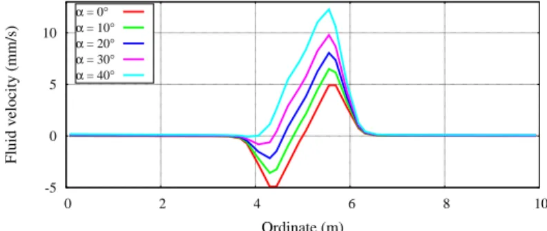
Figure 6: Tangential fluid velocity along the interface at steady state
initial defect
V0 p = 0
Figure 7: Geometry and boundary conditions of two–dimensional example problem
porosity nf = 0.3. Non-Uniform Rational B-Splines have been used for the spatial
discretisation, with the displacements interpolated by cubic splines and the pressure interpolated by quadratic splines [23]. Matching interface elements have been used to model the (stationary) discontinuity.
Figure 5 shows the effects of the flow in the cavity on the area surrounding the cav-ity at an early stage of the simulation. When the term for the flow in the discontinucav-ity is made inactive, the flux is the same at both faces of the discontinuity, i.e. the fluid flows through the cavity without being affected by it. The jump in the fluid flow is clear in the right part of Figure 5, with fluid being stored and flowing away within the cavity.
Figure 6 shows that for a horizontal crack (α=0), the fluid velocity is symmetric in the cavity, flowing to the left and to the right in equal amounts. When the interface is inclined, the fluid can accelerate in the cavity, which starts to behave like a resistance-free channel for the fluid.
4.2. Discontinuous pressure at the interface
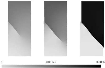
Figure 8: Evolution of the displacement field at t=18 s, 22 s, 26 s
V0 = −10−4m/s. The pore pressure at the top of the specimen is the reference
pres-sure, here zero, and undrained boundary conditions have been imposed on the other boundaries. The solid constituent is assumed to behave in a linear elastic manner with a Young’s modulus E =20 GPa and a Poisson’s ratioν=0.35. The Biot coefficient
αhas been set equal to 1, the Biot modulus has been assigned a value M =5.0 GPa, while the bulk material was assumed to have a permeability kf =10−14m3/Ns.
Shear-band formation was triggered by a small imperfection, see Figure 7. The critical shear stress at which nucleation occurred, was taken asτc = 100 MPa and after inception
the shear-band evolution is controlled by a mode-II fracture energy,GII
c = 500 J/m2.
In the example calculations, the permeability of the diaphragm has been assigned
knd =0.5·10−14m3/Ns, which is half of that in the bulk.
Different from the previous example, the specimen has been discretised with quadri-lateral basis elements with a bilinear Lagrange interpolation scheme for the displace-ments as well as for the pressure. This scheme is not optimal, but has been used to avoid complexities in the Extended Finite Element approach that has been adopted to model the propagating shear band, especially with respect to the integration of the dif-ferent parts of the load vectors and stiffness matrices in elements which are crossed by the discontinuity [10]. In the simulations, 24 elements have been used across the width of the specimen and 60 elements over the height. The simulation has been carried out in 65 equal time steps over a total time of 26 s.
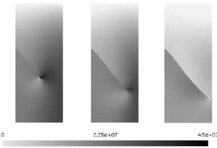
Figure 9: Evolution of the pressure field at t=18 s, 22 s, 26 s
The pressure distribution is strongly influenced by the propagation of the interface even in the present case where kf and kndare of the same order of magnitude. Indeed,
the pressure discontinuity is significant as observed in Figure 9. Accordingly, the rel-atively lower permeability at the discontinuity has a major influence on the fluid flow, and therefore on the stress distribution inside the specimen.
5. Concluding remarks
Acknowledgement
Financial support through the ERC Advanced Grant 664734 ”PoroFrac” is grate-fully acknowledged.
References
[1] J. G. Rots, Smeared and discrete representations of localized fracture,
Interna-tional Journal of Fracture, 51, 1991, 45–59.
[2] J. C. J. Schellekens and R. de Borst, On the numerical integration of interface elements, International Journal for Numerical Methods in Engineering, 36, 1993, 43–66.
[3] A. R. Ingraffea and V. Saouma, Numerical modelling of discrete crack propaga-tion in reinforced and plain concrete. In: Fracture Mechanics of Concrete, Marti-nus NijhoffPublishers, Dordrecht, 1985, 171–225.
[4] G. T. Camacho and M. Ortiz, Computational modelling of impact damage in brit-tle materials, International Journal of Solids and Structures, 33, 1996, 2899– 2938.
[5] B. A. Schrefler, S. Secchi and L. Simoni, On adaptive refinement techniques in multifield problems including cohesive fracture, Computer Methods in Applied
Mechanics and Engineering, 195, 2006, 444–461.
[6] S. Secchi, L. Simoni and B. A. Schrefler, Mesh adaptation and transfer schemes for discrete fracture propagation in porous materials, International Journal for
Numerical and Analytical Methods in Geomechanics, 31, 2007, 331–345.
[7] S. Secchi, B. A. Schrefler, A method for 3-D hydraulic fracturing simulation,
International Journal of Fracture 178, 2012, 245–258.
[8] T. Belytschko and T. Black, Elastic crack growth in finite elements with mini-mal remeshing, International Journal for Numerical Methods in Engineering, 45 (1999) 601–620.
[9] N. Mo¨es, J. Dolbow and T. Belytschko, A finite element method for crack growth without remeshing, International Journal for Numerical Methods in Engineering, 46 (1999) 131–150.
[10] R. de Borst, J. R´ethor´e and M.A. Abellan, A numerical approach for arbitrary cracks in a fluid-saturated porous medium, Archive of Applied Mechanics, 75, 2006, 595–606.
[11] J. R´ethor´e, R. de Borst and M.-A. Abellan, A two-scale approach for fluid flow in fractured porous media, International Journal for Numerical Methods in
[12] J. R´ethor´e, R. de Borst and M.A. Abellan, A discrete model for the dynamic propagation of shear bands in a fluid-saturated medium, International Journal for
Numerical and Analytical Methods in Geomechanics 31, 2007, 347–370.
[13] J. R´ethor´e, R. de Borst and M.A. Abellan, A two-scale model for fluid flow in an unsaturated porous medium with cohesive cracks, Computational Mechanics, 42, 2008, 227–238.
[14] F. Irzal, J. J. C. Remmers, J. M. Huyghe and R. de Borst, A large deformation formulation for fluid flow in a progressively fracturing porous material, Computer
Methods in Applied Mechanics and Engineering, 256, 2013, 29–37.
[15] T. Mohammadnejad and A.R. Khoei, Hydro-mechanical modelling of cohesive crack propagation in multiphase porous media using the extended finite element method, International Journal for Numerical and Analytical Methods in
Geome-chanics, 37, 2013, 1247–1279.
[16] T. Mohammadnejad and A.R. Khoei, An extended finite element method for fluid flow in partially saturated porous media with weak discontinuities: the con-vergence analysis of local enrichment strategies, Computational Mechanics, 51, 2013, 327–345.
[17] B. Carrier and S. Granet, Numerical modelling of hydraulic fracture problem in permeable medium using cohesive zone model, Engineering Fracture Mechanics, 79, 2012, 312–328.
[18] F. Armero and C. Callari, An analysis of strong discontinuities in a saturated poro-plastic solid, International Journal for Numerical Methods in Engineering, 46, 1999, 1673–1698.
[19] J. M. Segura and I. Carol, Coupled HM analysis using zero-thickness interface elements with double nodes. Part I: Theoretical model, International Journal for
Numerical and Analytical Methods in Geomechanics, 32, 2008, 2083–2101.
[20] J. M. Segura and I. Carol, Coupled HM analysis using zero-thickness inter-face elements with double nodes. Part II: Verification and application,
Interna-tional Journal for Numerical and Analytical Methods in Geomechanics, 32, 2008,
2103–2123.
[21] J. Larsson and R. Larsson, Localization analysis of a fluid-saturated elastoplas-tic porous medium using regularized discontinuities, Mechanics of
Cohesive-frictional Materials, 5, 2000, 565–582.
[23] J. Vignollet, S. May and R. de Borst, Isogeometric analysis of fluid-saturated porous media including flow in the cracks, International Journal for Numerical
Methods in Engineering, 2016, DOI: 10.1002/nme.5242.
[24] R. de Borst, M. A. Crisfield, J. J. C. Remmers and C. V. Verhoosel, Non-Linear
Finite Element Analysis of Solids and Structures, Second Edition, Wiley & Sons,
Chichester, 2012.
[25] J. M. Segura and I. Carol, On zero-thickness interface elements for diffusion problems, International Journal for Numerical and Analytical Methods in
Ge-omechanics, 28, 2004, 947–962.
[26] E. W. Remij, J. J. C. Remmers, J. M. Huyghe and D. M. J. Smeulders, The enhanced local pressure model for the accurate analysis of fluid driven fracture in porous materials, Computer Methods in Applied Mechanics and Engineering, 286, 2015, 293–312.
[27] R. W. Lewis and B. A. Schrefler, The Finite Element Method in the Static and
Dy-namic Deformation and Consolidation of Porous Media, Second Edition, Wiley
& Sons, Chichester, 1998.