Simulation Of Displacement Control For Piezoelectric Actuator Using PID Controller (electronic resource)

SIMULATION OF DISPLACEMENT CONTROL FOR

PIEZOELECTRIC ACTUATOR USING PID CONTROLLER

MOHAMAD RAZIF BIN MOHD JABAR

B050910010

UNIVERSITI TEKNIKAL MALAYSIA MELAKA

SIMULATION OF DISPLACEMENT CONTROL FOR

PIEZOELECTRIC ACTUATOR USING PID CONTROLLER

This report submitted in accordance with requirement of the Universiti Teknikal Malaysia Melaka (UTeM) for the Bachelor Degree of Manufacturing Engineering

(Robotic and Automation) (Hons.)

by

MOHAMAD RAZIF BIN MOHD JABAR

B050910010

870328-23-5401

UNIVERSITI TEKNIKAL MALAYSIA MELAKA

BORANG PENGESAHAN STATUS LAPORAN PROJEK SARJANA MUDA

TAJUK: Simulation of Displacement Control For Piezoelectric Actuator Using PID Controller

SESI PENGAJIAN: 2012/13 Semester 2

Saya MOHAMAD RAZIF BIN MOHD JABAR

mengaku membenarkan Laporan PSM ini disimpan di Perpustakaan Universiti Teknikal Malaysia Melaka (UTeM) dengan syarat-syarat kegunaan seperti berikut:

1. Laporan PSM adalah hak milik Universiti Teknikal Malaysia Melaka dan penulis. 2. Perpustakaan Universiti Teknikal Malaysia Melaka dibenarkan membuat salinan

untuk tujuan pengajian sahaja dengan izin penulis.

3. Perpustakaan dibenarkan membuat salinan laporan PSM ini sebagai bahan pertukaran antara institusi pengajian tinggi.

(Mengandungi maklumat yang berdarjah keselamatan atau kepentingan Malaysia sebagaimana yang termaktub dalam AKTA RAHSIA RASMI 1972)

(Mengandungi maklumat TERHAD yang telah ditentukan oleh organisasi/badan di mana penyelidikan dijalankan)

TIDAK TERHAD

Alamat Tetap:

No 180 Kampung Belahan Tampok

83100 Rengit, Batu Pahat

Johor Darul Takzim

Tarikh: ________________________

Disahkan oleh:

Cop Rasmi:

Tarikh: _______________________ 4. **Sila tandakan ( )

SULIT

DECLARATION

I hereby, declared this report entitled “Simulation of Displacement Control for Piezoelectric Actuator using PID Controller” is the results of my own research

except as cited in references

Signature : ---

APPROVAL

This report is submitted to the Faculty of Manufacturing Engineering of UTeM as a partial fulfillment of the requirements for the degree of Bachelor of Manufacturing Engineering (Robotics and Automation) (Hons.). The member of the supervisory committee is as follow:

ABSTRAK

ABSTRACT

DEDICATION

ACKNOWLEDGEMENT

I would like to thank Encik Mohd Nazmin bin Maslan for being a wise supervisor of the project. His wonderful conduct, aware criticisms and patient support the writing of the report in inestimable ways. His support of the project was greatly needed and deeply be pleased about.

TABLE OF CONTENT

Abstrak i

Abstract ii

Dedication iii

Acknowledgement iv

Table of Content vii

List of Tables viii

List of Figures x

List Abbreviations, Symbols and Nomenclatures xi

CHAPTER 1: INTRODUCTION 1

1.1 Background 2

1.2 Problem Statement 3

1.3 Objectives 3

1.4 Scope of the Study 4

1.5 Summary 4

CHAPTER 2: LITERATURE REVIEW 5

2.1 Introduction 5

2.2 Piezoelectric 6

2.3 Piezoelectric Actuator 6

2.3.1 Patch Actuator 7

2.3.2 Bender Actuator 8

2.4 Displacement Application Control System 9 2.4.1 Closed Loop System 10

2.5 System Identification 11

2.6.1 Proportional Controller 13 2.6.2 Integral Controller 13 2.6.3 Derivative Controller 14

2.7 Controller Parameter 15

2.8 Summary 16

CHAPTER 3: METHODOLOGY 17

3.1 Introduction 17

3.2 Problem Analysis 18

3.3 Project Flow Chart 19

3.3.1 Final Year Project 1 20 3.3.2 Final Year Project 2 21

3.4 Project Planning 23

3.5 Programming Flow Chart 24

3.6 Experimental Setup 26

3.7 Method of Controller Setup 26

3.8 Heurestic Method 28

3.9 SISO Design Tool 29

3.9.1 SISO Tool Design Flowchart 30 3.9.2 PID Controller Parameter Using SISO Tool 38

3.10 Summary 39

CHAPTER 4: RESULTS AND DISCUSSION 40

4.1 Introduction 40

4.5.1 Simulation Results for Heurestic Method 54 4.5.2 Simulation Results for SISO Tool 60 4.6 Comparative Study and Discussion 62

4.6 Overall Discussion 63

CHAPTER 5: CONCLUSION 64

5.1 Conclusion 65

5.2 Future Works 66

REFERENCES

LIST OF TABLES

2.1 Setup the Parameter of Controller 15

3.1 Gantt Chart 23

3.2 The Requirement Range for Phase Margin and Gain Margin 29

LIST OF FIGURES

1.1 Closed Loop System 2

2.1 Design Principle of Patch Actuator 7 2.2 Closed Loop Bender Actuator 8 2.3 Designs for Closed Loop System 10 2.4 Procedure of System Identification Technique 11 2.5 Proportional Controller in Closed Loop System 13 2.6 Integral Controller in Closed Loop System 13 2.7 Derivative Controller in Closed Loop System 14

3.1 Problem Analysis Flow Chart 18

3.2 Project Flow Chart 19

3.3 Fina1 Year Project 1 20

3.4 Fina1 Year Project 2 21

3.5 Programming Flow Chart 24

3.6 Experimental Setup 25

3.7 Heurestic Method Flow Chart 28

3.8 Current Architecture 29

3.16 Controller Parameter for PID Controller for Patch Actuator 36 3.17 Export Compensator to the Workspace 37 3.18 PID Values for Patch Actuator 38 3.19 PID Values for Bender Actuator 38

LIST OF ABBREVIATIONS, SYMBOLS AND

NOMENCLATURE

Amp - Amplifier P - Proportional I - Integral D - Derivative

AFM - Atomic Force Microscopy DC - Direct Current

PLC - Programmable Logic Controllers DCS - Distributed Control Systems KP - Proportional Gain

KI - Integral Gain KD - Derivative Gain PC - Personal Computer m. - Matlab Files

u - Volume Velocity

t - Time Variable

r - Reflection Coefficient or Radius

τ - Delay

d - Fractional Part of the Total Delay D

e - Vector of Complex Exponentials - Integral

CHAPTER 1

INTRODUCTION

1.1 Background

Piezoelectric actuators are electromechanical device and energy transducer between electrical and mechanical that will produce a value of voltage. The piezoelectric actuators are available for managing small displacements in the certain range. The characteristic of the piezoelectric actuator is fast response, low tear and wear and high stiffness.

Descriptions regarding to piezoelectric actuator, this device is used for high precision mechanical and electrical engineering applications. Many researchers have found that some useful applications for piezoelectric such as detection of sound, electronic frequency and ultrafine focusing of optical assemblies. These applications are used widely in many fields of industrial production. The piezoelectric actuators also used in the structural system to control noise, vibration and shape. The element of piezoelectric in complex actuator can be integrated in robotics design affecting the structural properties of the whole system. Manufactured on the stacking up piezoelectric disks or plates is the application that actuator configuration depend on and when the voltage being applied, the axis of the stack being the axis of linear motion.

In the shape of planar disk, the device such as disk actuator is used. Disk actuators are called a ring actuator with center bore that make axis of the actuator are accessible for mechanical, electrical or optical purposes. Bimorph styles, block, disk, and bender are included in the common configurations.

However, piezoelectric actuator can also be implemented as an ultrasonic device. The piezoelectric device is used especially for controlling the positioning application, quick switching and vibration. Either amplified or direct is the function of piezoelectric actuator. The force in piezoelectric actuator is needed to elongate to the certain amount.

There are several controllers in control system such as: 1. Proportional controller

2. Derivative controller 3. Integral controller

They are simply gaining value in the proportional controller. This controller is a multiplication coefficient. For controlling based and future values where the signal is going to be in the future, the derivative controller is implemented to account. The integral controller can add up the area under the curve for the past time. This controller can correct based on past errors. Figure 1.1 illustrates an example of a closed loop system that equips with the controller.

1.2 Problem Statement

The piezoelectric had inaccuracy behavior to maintain the displacement output from the transfer function given. This project is to control the displacement of piezoelectric actuator using the suitable controller. To choose the suitable controller, we must define the range of PID controller gains on an open loop and closed loop system.

For piezoelectric actuators, first, compare the types of actuators that had existed such as bender and patch, each with their own transfer function. The range of the laser displacement that attach will be determined also based on piezoelectric actuators.

From the previous studies, there are several characteristic of piezoelectric actuators that has such ability to create high forces, a high efficiency, high mechanical durability and short response time. Piezoelectric actuators also have small strains and a high supply needed. This problem also needs to determine the values of controller parameter on piezoelectric actuator. The values of controller parameter will be obtained based on the range of the stability. In that case, the values for the controller parameter will determine by the method approach.

1.3 Objectives

The main objective of this project is to simulate and control the displacement from piezoelectric actuator. MATLAB software is used to create the open loop and closed loop system based on the transfer function from the piezoelectric actuators.

1. To compare and analyze the piezoelectric actuators, ie. Patch and bender.

1.4 Scope of the Study

The scope of the project was to compare and analyzes the piezoelectric actuators controller’s parameter function that related to open loop or closed loop system. Study the function and the characteristic of piezoelectric actuators such as patch and bender.

This project also focuses on the PID controller and defines the controller parameter such as Kp,Ki and Kd. This parameter will control the displacement for piezoelectric actuator and reduce the overshoot and also get the stable system for open loop and close loop. The transfer function for piezoelectric actuators is not stable and then adds the controller to control the displacement output.

1.5 Summary

CHAPTER 2

LITERATURE REVIEW

2.1 Introduction

For this project, the literature review had performed in order to simulate of displacement control for piezoelectric actuator using PID controller. This chapter also explored about the recent study of Control System and Matlab. The information, idea and knowledge were obtained from the journal, website, articles and books also as sources in order to complete this study.

2.2 Piezoelectric

From the history of piezoelectric actuator, in 1880, Jacques Curie and Pierre have discovered the effect of piezoelectric. Crystal symmetry and pyroelectricity has relations that led the brother. The relations not only identify pressure for electrification but also identify which crystal classes the effect expected and what direction pressure should apply. (Novotny & Ronkanen, 1997)

Before the end of 1881, Curies has verified this term. The effect of the inverse of piezoelectric is the application of the electric field to the crystal piezoelectric has to lead a deformation of physical for the crystal. Piezoelectric ceramic was discovered in the year 1950. The effect of piezoelectric ceramic is much stronger. The polarizing process is the process that undergoes the piezoelectric ceramics and the crystal materials are natural. (Novotny & Ronkanen, 1997)

For the hysteresis of non-linearity behavior, the output displacement yields and input voltage are an independent lag and the residual displacement has near to zero. The non-local memory always effect by the hysteresis between output and input of non- linearity. There are several methods exist to reduce the hysteresis non-linearity of the piezoelectric. This method based on the linear mapping between the driving charge and the displacement of the piezoelectric. (Tzen, et al. 2003)

2.3 Piezoelectric Actuator

2.3.1 Patch Actuator

Figure 2.1: Design Principle of Patch Actuator (Physik Instrumente, 2011)

2.3.2 Bender Actuator

Usually, bender actuators are used in many applications such as Atomic Force Microscopy (AFM), force sensor, positioning devices and cantilevers. The process of optimization and design needs numerical and analytical modeling to achieve the desired performance. In the numerical modeling like finite element of analysis, the behavior will shows by the given structure. The analytical model will allow the various parameters in systematic optimization. The tools in finite element can handle the parametric models and can be used to optimize and design piezoelectric benders. To achieve and justify the analytical model, the model characteristic must far and more adaptable to the input parameter. The materials and geometry principle are the example as the corresponding numerical model. (Dunsch & Breguet, 2007)

Figure 2.2: Closed Loop Bender Actuator (Physik Instrumente, 2011)

2.4 Displacement Application Control System

From the previous study, the displacement application in a control system is applied for canceling the control of displacement in the system of vibration isolation. A method to control that achieved infinite stiffness to direct disturbance is applied to a vibration isolation system. A method of this study is when the mass in the middle that has a spring connected from the base is suspended. The mass is the middle is displaced in the same direction of the force when the direct vibration acts on the isolation table. To cancel the displacement of the mass in the middle of the base, the actuator will operate to move to the isolation table in the opposite direction. A fabricating of the single axis apparatus will be done to verify the effect of this principle.(Mizuno et al. 2007)

Another DC motor installed between the mass which is the middle and base and also implemented with a controller such as I-PD controller for realizing displacement cancellation. The control method of the efficacy is experimentally and confirmed. (Mizuno et al., 2007)

Another case study for displacement in a control system is to develop a displacement fluid power system. This system uses the similar component as a load sensing system but the pump is controlled in different ways. The mode of the pressure is a close loop control but the pump operates in an open loop control mode. This principle might increase the energy efficiency, faster the response and less the oscillation. The displacement controlled is the pump and the valve is equipped with common pre compensators the flow delivered from the pump needs to be matched by the valve. The displacement controlled system has been designed and simulated using the AME simulation software. This system has been attached in a wheel loader application and it compared to a load sensing system. (Andersson, 2009)

2.4.1 Closed Loop System

In open loop systems, there are several disadvantages such as sensitivity to disturbance and inability to correct the disturbances may be solved in a closed loop system. The input for transducer will converts the form of the input to use in the controller. The output in transducer will measure the output response and converts to use by the controller. For example, from the previous experiment, if the controller uses electrical signals to make operation of the valves of a temperature in control system, the output temperature and input position are converted to electrical signals. (Norman S. Nise 2004)

Feedback

Figure 2.3: Design for Closed Loop System

The summing junction adds the signal from the input to the signal from the output and arrives by the feedback path and the return path from the output of the summing junction. The output signal is subtracted from the input signal. The result from the output is called the actuating signal. Measuring the output response, feeding measurement back through a feedback path and comparing the response to the input at the summing junction by closed loop system will compensate for disturbances. If the two responses have any difference, the system will drives the plant by actuating signal to make the correction in the system. If there is no difference between the two responses, the system does not drive the plant, since the plant’s response has been already the desired response. In the closed loop system, it is less sensitive to noise, disturbances and changes in the environment rather that open loop system. (Norman S. Nise, 2004)

The steady-state error and the transient response can be controlled more conveniently and with greater flexibility in a closed loop system by a simple adjustment of gain in the loop and sometimes by redesigning the controller. The closed loop systems are expensive and more complex than an open loop system. (Norman S. Nise, 2004)

The advantages of feedback control are to keep the variable process close to the nearest value wherever have disturbances and variation from the process. The lower cost in control system has increased the applications of the feedback principle. (Norman S. Nise , 2004)

2.5 System Identification

2.6 PID Controller

A proportional integral derivative (PID) controller is the controller that has a history in the control system. This controller is able to provide a wide range of processes and also has been applied with a progress of technology that implemented in digital form rather than pneumatic and hydraulic components. This control equipment as a standalone controller and was added to functional block such as Programmable Logic Controllers PLC) and Distributed Control Systems (DCS). In the PID controller, the new effective tools have been added for improving the analysis and design methods in the basic of algorithms in order to increase the performance. (Antonio Visioli, 2006)

2.6.1 Proportional Controller

The first term in PID controller is proportional controller. This proportional controller is used to control the error according to the equation of Kp. The equation of Kp is shown below:

u(t) = Kpe(t) = Kp(r(t) - y(t)), (2.1)

Figure 2.4: Proportional Controller in Closed Loop System

2.6.2 Integral Controller

The integral controller is used to proportional to the integral of the control error. The value of Ki is the integral gain. This integral action is related to the past values of the control error. The transfer function for the Ki is shown below.

(2.2)

2.6.3 Derivative Controller

Proportional action based on the current value of the control error, the integral action is based on the past values of the control error and the derivative action is based on the future values based on predictions of the control error. The control law of derivative controller has shown below:

(2.3)

The derivative controller has a great potential in improving the control performances. This controller also counteracts an incorrect trend of the control error. On some issues, this derivative controller not very frequently adopted. (Antonio Visioli, 2006)

2.7 Controller Parameter

In the PID controller, the certain value that is added to a controller parameter will change the output of the transfer function. There are four major characteristics of the closed loop system that will affect the system:

1. Rise time 2. Overshoot 3. Settling time 4. Steady-state error

Firstly, the rise time is the time that takes for the plant output y rise beyond 90% of the desired level for the first time. Then, the overshoot is to find the values at the peak level and compare if the values at the peak level is higher than the steady state or normal against the steady state. The settling time is the time that takes for the system collect to its steady state. Finally the steady-state error is to define the difference between the steady-state output and the desired output. The Table 2.1 shown below the setup for the parameter controller. (Jinghua Zhong , 2006)

Table 2.1: Setup the Parameter of Controller

Response Rise Time Overshoot Settling Time Steady-State

Error

Kp Decrease Increase NT Decrease Ki Decrease Increase Increase Eliminate Kd NT Decrease Decrease NT

2.8 Summary

CHAPTER 3

METHODOLOGY

3.1 Introduction

In this chapter of methodology, it discussed on how to carry out this study that is focused on how to identify the desired objectives through the selected tools. This chapter is to cover the methodology from the project planning, project flow chart, product case study and design the flow chart that to achieve the objectives.

3.2 Problem Analysis

The problem analysis is to define the problems that appear that should solve in this project. The purposes of this project are to solve the error on the system by using the experimental project. This project needs to identified, analyze and focus on the key word that has identified such as:

1. MATLAB & SISO Tool 2. PID controller

The flow of problem analysis is used to find the problem that stated above. That keyword is related to the objective that has identified.

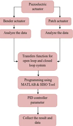
Piezoelectric actuator

Bender actuator Patch actuator

Analyze the data Analyze the data

Transfers function for open loop and closed

loop system

Programming using MATLAB & SISO Tool

PID controller parameter

Collect the result and data

3.3 Project Flow Chart

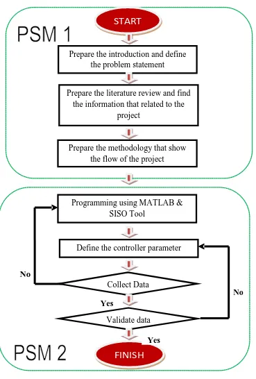
The project flow chart was to describe the flow of the activities involve in the project from the beginning till the end project. The project flow chart was shown in Figure 3.2.

START

Prepare the introduction and define the problem statement

Prepare the literature review and find the information that related to the

project

Prepare the methodology that show the flow of the project

Programming using MATLAB & SISO Tool

Define the controller parameter

No

Collect Data

No Yes

Validate data

3.3.1 Final Year Project 1

In the beginning of the research that shows in the Figure 3.2, this research aims to and understand the importance and basis of research that define the problem statement and the objectives of the study. This main objective of this project was to simulate and control displacement from piezoelectric actuator. This stage was the critical phase in determining the scope and significance of the study towards achieving highly anticipated results. The objective and the scope must be identified clearly to make sure to get maximum and a clear understanding about the topic.

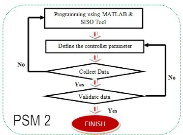
3.3.2 Final Year Project 2

In this stage of research that shows in Figure 3.4, there is the important stage that should clearly define and understand the outcome of this project. The programming is the stage that design to give the instruction and communicate with the machine. Then, the programming will transfer to the real application to prove the objective. The purposes that build a program on PID controller are to control the displacement of the experimental project.

3.4 Project Planning

The project planning is to explain and develop this report. In the PSM 1, it explains about introduction, literature review, methodology, preliminary result and conclusion that should be done during semester 1. In the PSM 2, it explains about results and discussion that should do during semester 2.

In the PSM 1, the introduction more focused on the background of study, objectives, scope of study and problem statement. A literature review was focused about previous research and case study that related to this project. All the sources and references have been found from the journals, books, website, and articles. The methodology reviews about the flow of the project, the planning of this project, the flow to develop programming using MATLAB software that will integrate to the experimental rig. The preliminary results discuss about the expected finding about this project. The method to determine the parameter gains such as Kp, Ki and Kd. Find the case study about the step response that will prove the advantages using the PID controller. The conclusion will conclude about the work that have done in PSM 1 and the future work that will be done in PSM 2.

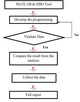
3.5 Programming Flow Chart

The research of this project continues with the programming stage. This stage is to instruct and do the simulation from the m.file and SISO tool. Develop the programming using MATLAB because this software is built to define the open loop and closed loop transfer function. The parameter of the controller that gets from the SISO tool will compare to the trial and error method and justify the better values. This must be synchronized well to make the project run perfectly. The data that is collected based on the peak response and the rule of thumb. The figure 3.5 shows the programming flow chart.

MATLAB & SISO Tool

Develop the programming

Validate Data

Yes

Compare the result from the analysis

Collect the data

Full report

3.6 Experimental Setup

In the experimental setup, all the data that collected from the experiment were assessed using a laser sensor and fixed with a module jig to measure the displacement signal. The personal computer were recorded the displacement signals at a sampling rate of 1 kHz using a 16-bit PCI Data Acquisition Card (DAQ). LabVIEW software was used to data processing and routines analysis. After 10 seconds, the program will automatically terminate. DAQ will supply by 10 volt Hz triangle-wave. The actuators set of amplifiers that will amplify the voltage to 60 V. A series voltage was applied to piezoelectric actuator that enables it to freely displace its active elements at its free end with the other end fixed. Low frequency (10 Hz) input wave form used to reduce the dynamic effect. The MATLAB used as the main programming environment for executing the SI command lines. MATLAB program has created refer to RLS using ARX model. When transfer function has been determined, the result will verified and validated via modeling and simulation using MATLAB. Figure 3.6 show the experimental setup for the piezoelectric actuator. (Maslan M. N., 2012).

Below is the transfer function for patch actuator that defines using system identification. (Maslan M. N., 2012).

3.1

Below is the transfer function for the bender actuator that defines using system identification. (Maslan M. N., 2012).

3.2

3.7 Method of Controller Setup

The PID controller setup is to describe about the methods of the beginning to use the PID controller. The method of this PID controller is very important because without the systematic method about the PID controller, it's very difficult to define the values of the proportional, integral and derivative. The method in controller setup will show step by step how to gain parameter in Kp,Ki and Kd in PID controller.

3.8 Heuristic Method

In MATLAB software, several methods are used to design a PID controller. The trial and error method usually use in MATLAB to create a coding in the command window. This method is the basic method to design any coding that related to the PID controller or any calculation in mathematics. To ease in use this command window to create coding, use the editor in MATLAB that can fix the error of the coding. The error such as missing any command can be easily fixed.

The error command can be red line and the editor can detect it. The trial and error method is the method that inserts any values of KP, Ki and Kd in design controller based on the transient response and Bode diagram.

The numerator and denominator are to model the transfer function. The numerator is the number or expression above the fraction bar and the denominator is the number or expression below the fraction bar. The parameter value will define using trial and error that inserts any value of Kp, Ki and Kd.

Start

Declare plant for the patch and bender

Declare input for time delay and converter

Insert the parameter value for Kp, Ki and Kd

Validate Data

Yes

End

Figure 3.7: Heurestic Method Flow Chart

No

3.9 SISO Design Tool

SISO Tool is the Graphical User Interface that lets to design single input and single output (SISO) that compensators by graphically interacting with the root locus, Bode and Nichols plots of the open loop system.C and F are tunable compensators. SISO tool (G) specified the plant model G to be used in the SISO Tool. Here G is any linear model created with TF, ZPK, or SS. (G, C) and (G, C, H, F) further specify values for the feedback compensator C, sensor H, and prefilter F. By default, C, H, and F are all unit gains. The current architecture is shown below:

F

C

G

H

Figure 3.8: Current Architecture

Table 3.2: The Requirement Range for Phase Margin and Gain Margin

Requirements

Phase Margin

Gain Margin

Range

3.9.1 SISO Tool Design Flowchart

The SISO Tool Design Flowchart will show step to use the SISO tool toolbox in MATLAB software. The result will show the graph based on the values on the Kp, Ki and Kd in parameter of controller.

Start

Design the coding for patch and bender

Import the G(s) and PID formula

Adjust the zero and poles at the open loop Bode diagram

Calculated the value Kp, Ki,and Kd using coding

Validate Data

Yes End

Figure 3.9: SISO Design Tool Flow Chart

3.9.2 PID Controller Parameter Using SISO Tool

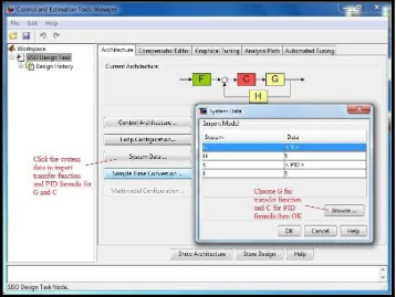
The toolboxes of SISO tool will appear on screen. The coding used the MATLAB that has defined the transfer function, converter and time delay must be run first in the command window. Then, open the system data in the SISO Tool toolbox to import the G(s) of the transfer function and the formula of the PID controller.

The Nyquist diagram, Bode diagram for open loop and close loop were generated and the expected parameter value of the PID controller will define based on the range of phase margin and gain margin. The coding to design patch actuator and bender actuator were generated to the command window that show in Figure 3.11 and Figure 3.12. These two transfer functions were imported of the system data and also the PID formula that shows in Figure 3.13.

Figure 3.12: Programming for Bender Actuator

In Figure 3.14 show the SISO design simulation for the patch actuator and Figure 3.15 show the SISO design simulation for the bender actuator. The brown dot at the open loop Bode diagram will be adjusted. The brown dot is the zero of the transfer function. The zeros will be adjusted based on range of phase margin and the gain margin to get the stable loop. Sometimes, the phase margin and gain margin in the range but the transfers functions stability remains in an unstable loop. This case likely behavior of the electromechanical devices is non-linear.

The Bode diagram for phase margin and gain margin can be zoomed out and zoom in to look closely on the zeros. This action is the way to get better values for the phase margin and the gain margin. Bode diagram on the left show the stability for the transfer function of patch actuator and bender actuator. The value of the peak response of the closed loop transfer function can be determined at the Bode diagram.

Figure 3.15: SISO Design for Bender Actuator

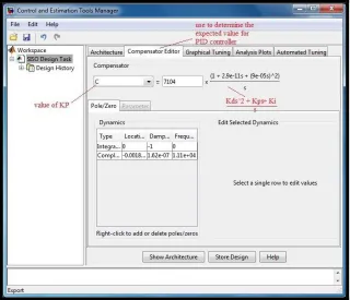
The Control and Estimation Tool Manager is the tool to determine the expected value of Kp, Ki and Kd, show the result by the graph of Bode diagram and Nyquist plot and so on. Compensator Editor will view the value of Kp, Ki and Kd. The value of KP, Ki and Kd are getting after the value of phase margin and gain margin are determined after adjusting the graph. The C represents the value of Kp. The value of Kp will multiply the value of Ki and Kd using the coding. The value will be exported to the command window.

Figure 3.16: Controller Parameter for PID Controller for Patch Actuator

The value of C at the Compensator Editor will be chosen and then export to the workspace. Figure 3.18 shows the compensator value export to the workspace. The programming will be made to calculate the value of Kp, Ki and Kd. Insert the value of Kp,Ki and Kd to the coding of PID controller that create by m.files in the command window. The result should be same as the SISO Tool method.

Figure 3.18: Export Compensator to the Workspace

After the values of compensator export to the workspace, write the coding for the PID controller and the transfer function of feedback controller will generate. The value for Kp, Ki and Kd will appear in the transfer function. Collect the values for the result by using the SISO Tool method. Figure 3.19 and Figure 3.20 shows the transfer function and also the value for the Kp, Ki and Kd.

Figure 3.19: PID Values for Patch Actuator

3.9 Summary

The methodology shows all the flow about the final year project for semester 1 and semester 2. The project planning shows the plan from the beginning of the project until the project finish. All the planning is designed to achieve the objectives. In the problem analysis,

CHAPTER 4

RESULTS AND DISCUSSION

4.1 Introduction

This chapter consists the result and discussion that get from the project through the methodology in chapter 3. This topic will discuss about the advantages and disadvantages of the PID controller. This main problem that occurred to finish this project is to set up the PID controller in programming and the control box. This chapter also discusses about case study related to the comparison of using PID controller and without using PID controller. In closed loop system, this system will equip with PID controller and without the PID controller to compare the end result of the project. The several benefits using this PID controller are this controller can correct the error of the past and stable the transfer function from the piezoelectric actuators.

4.2 Design Structure for Controller

All these components is the requirement to model the unique transfer function for the patch actuator and bender actuator. Both of these electromechanical actuators are difficult to control because of their inherent nonlinearity and hysteresis. According to the research, if voltage input voltage is applied to piezoelectric actuator and their relation can be linearized as a second-order linear dynamic system. The Figure 4.1 will show the relationship between voltage u and displacement y.

Figure 4.1: One Degree of Freedom Control Configuration

The block diagram that is shown above is the structure of the one degree of freedom for close loop transfer function. The r is the input of the system. The component of the input such as step input that suitable for close loop system. The K is a value parameter for the gain in PID controller. The value of this controller usually can get used heuristic method and SISO tool. The u is the command control signal that brings the impact to the input and error. G represents the transfer function from the patch actuator and bender actuator. Then y,is the output of the system of open loop or close loop depend on the system that is created. Lastly, ym is the feedback from the output to the input for the close loop system. For a continuous time system, G relates to the Laplace transform of the input

u(s) and the output y(s) as follows

4.2.1 Design Structure for Patch Actuator

In this design structure, the transfer function that gets from patch actuator will be modelled to define the expected parameter value for the KP, Ki and Kd. The transfer function is defined from the data that is collected from the experimental rig. The possibility of the transfer function that is not stable is high because the patch behavior is non-linearity. All data capturing experiments were assessed using a displacement laser and fixed with a module jig to measure the displacement signal. Then, the transfer function has been calculated based on the RLS method. Transfer function for the patch is in second order system. These transfer functions maybe have the unstable system. (Maslan M. N., 2012)

4.2.2 Design Structure for Bender Actuator

The design of bender actuator is almost similar from patch actuator. The transfer function that gets from bender actuator will be modelled to define the expected parameter values for KP, Ki and Kd. The PID controller will be used to control the displacement of the actuator. The data will be collected from experimental rig to form the transfer function. The RLS method has been used to define the transfer function for bender actuator. The non-linearity behavior of bender makes the possibility of the transfer function not stable is high. The transfer function for bender is in second order system. The displacement of bender actuator will be controlled using suitable method

4.3 Analysis of the MATLAB Code for Patch Actuator

In heuristic method, the manual programming will create on the command window. The coding will create based on the transfer function from patch actuator. The trial and error method will be used to determine the parameter values for Kp, Ki and Kd. Usually, values for Kp is larger than Ki and Kd. Estimated the parameter values for Kp, Ki and Kd between the range of phase margin and the gain margin. The parameter values also refer to the stability that will be plotted on Bode diagram and Nyquist. The transfer function G(s) for the patch actuator is:

G(s) = 0.03747 s^2 -0.07066 s + 0.03319 (4.2) 0.4882 s^2 -1.492 s + 0.0039

Declare the transfer function that defines as numerator and denominator. The transfer function is on the second order system. The numerator is (0.03747 -0.07066 0.03319) and the denominator will substitute a = 0.4882, b = -1.492, and c = 0.0039 into equation of G(s).

num = [0.03747 -0.07066 0.03319];

a = 0.4882;

b = -1.492;

c = 0.0039;

G = tf(num,[a b c]);

Equation (delay_tf) should be changed in the form of the transfer function and multiply by transfer to patch actuator G(s).

[num,den] = pade (0.00065,2);

delay_tf=tf(num,den);

The transfer function is in unit voltage. The converter is put to convert the voltage to the displacement unit. The command is:

P = (250/100);

Transfer function for the patches G(s) that have been issued then multiplied by the transfer function for the time delay (delay_tf). Then, total value for the transfer function (G_delay) multiplied by the converter (P) to convert the unit voltage to displacement.

G_delay= G*delay_tf;

V = G_delay*P;

During designing a PID controller, the objectives are finding based on the controller parameter which are Kp, Ki and Kd. The controller parameters are obtained using trial and error method. The parameter values for PID controller are Kp = 0.99, Ki = 10000, and Kd = 0.00035.

Kp= 0.99;

Ki= 10000;

Kd= 0.00035;

After define equation for the PID controller, MATLAB will calculate the equation with the value of Kp, Ki and Kd as determined earlier.

(L) is defined as open loop system. The (PID) equation will multiply to the (G_delay). In other words, a plot for Bode diagram is drawn and the Nyquist is plot for view a stability in imaginary axis.

L=(PID*V);

figure(1);margin(L);

figure(2);nyquist(L);

(T) define the close loop transfer function (20 log 10) plots at Bode diagram. The H = 1 in the feedback closed loop system.

T=feedback(L,1);

figure(3);Bode(T);

4.4 Analysis of the MATLAB Code for Bender Actuator

Trial and error is approached in the manual programming to obtain the parameter values for PID controller. The coding will create based on the transfer function from bender actuator. Usually, values for Kp is larger than Ki and Kd.

Estimated the parameter values for Kp, Ki and Kd between the range of phase margin and the gain margin. The parameter values also refer to the stability that will be plot on Bode diagram and Nyquist. The transfer function G(s) for the bender actuator is:

Plant transfers function that defines as numerator and denominator. The transfer function for bender is on the second order system. The numerator is (0.211 -0.2131 0.0021) and the denominator will substitute a = 0.1348, b = -1.13, and c = -0.0048 into equation of G(s).

num =[0.211 -0.2131 0.0021]

a = 0.1348;

b = -1.13;

c = -0.0048;

G = tf(num,[a b c])

Bender actuator also has a behavior of non-linearity same as patch actuator. The time delay (0,00065) will delay the response in output of transfer function. Syntax (pade) approximates time delays by rational models. Such approximations are useful to model time delay effects such as transport and computation delays within the context of continuous-time systems. Equation (delay_tf) changed in the form of the transfer function and multiplies by transfer to bender actuator G(s).

[num,den] = pade (0.00065,2)

delay_tf=tf(num,den)

The transfer function is in unit voltage. Insert the converter to convert the unit of voltage to the displacement. Define the command as:

P = (60/160)

Transfer function for the bender actuator G(s) have been obtained. Then, multiply the transfer function with the time delay (delay_tf).

Then, total value for the transfer function (G_delay) multiplied by the converter (P) to convert the unit of voltage to displacement.

V = G_delay*P

For the controller setting, parameter value of PID controller will find based on the controller parameter which are KP, Ki and Kd. The controller parameters are obtained using trial and error method. The parameter values for PID controller are Kp = 0.05, Ki = 11, and Kd = 0.00005.

Kp= 0.05;

Ki= 11;

Kd= 0.00005

Define equation for the PID controller and MATLAB will calculate the equation with the value of Kp, Ki and Kd that was obtained using trial and error method.

s=tf('s');

PID=tf(Kp + Ki/s + Kd*s);

Open loop system has defines as (L). The (PID) equation will multiply to the (G_delay). A plot for Bode diagram is drawn and the Nyquist is plot for view stability in imaginary axis for open loop system.

L=(PID*V);

figure(1);margin(L);

Close loop transfer function (T) for (20 log 10) plots at Bode diagram. From the feedback, H = 1. Plot the feedback in Bode diagram to obtain the value of peak amplitude.

T=feedback(L,1);

Figure (3); Bode (T);

4.5 Parameter for Controller

In parameter for the controller, it will explain about open loop control and close loop control. For open loop control, there is no use any kind feedback. If the system has an error, the open loop system can’t do anything. For close loop system is aimed the position and the best method to make the error of possibility zero.

In PID controller, proportional gain is immediate response to error but will not eliminate the error completely. The error will reduce by a small amount. Integral gain is working to remove small errors that proportional gain can’t do. Then, the derivative gain is related to the damping effect. In the real world, the derivative gain is a brake on the system of the car and the proportional is an accelerator.

4.5.1 Simulation Results for Heurestic Method

During designing a PID controller, the objectives are finding based on the controller parameters which are KP, Ki and Kd. The parameters of PID are obtained by a heuristic approach using trial and error.

Parameter Kp, Ki and Kd were selected based on the two requirement which are gain margin and phase margin are considered of the open loop transfer function. The range of gain margin and gain margin will ensure the stability for the system. Figure 4.2 and Figure 4.3 show the Bode diagram of open loop PID controller.

Figure 4.3: Bode Diagram of Open Loop System for Bender Actuator

For patch actuator, gain margin Gm = 7.21dB at frequency 505Hz and phase margin, Pm = 36º at frequency 278Hz and for bender actuator, gain margin Gm = 9.79dB at frequency 1.75e+03Hz and phase margin Pm = 49.3º at frequency 0.188Hz. The magnitude of gain margin and phase margin are in the range of the preferred consideration.

Nyquist diagram is plotted to verify the stability of PID controller. The gain and phase frequency are plotted in the Nyquist diagram to determine stability and performance. Bode plot are very useful tools in determining the system behavior at different sinusoidal excitation frequencies. Using gain margin and phase margin influence some limited stability insight is obtained for Bode plot. Plotting a Nyquist diagram and stability of the functional system is analyzed frequency domain based on the open loop transfer function. The system is stable because there are no encirclements at -1.

Figure 4.4: Nyquist Diagram for Patch Actuator

Figure 4.5: Nyquist Diagram for Bender Actuator

From open loop transfer function, a feedback has added to convert from the open loop transfer function into a close loop transfer function. From the close loop transfer function, Bode diagram is plotted to find bandwidth.

Bandwidth is the frequency at which magnitude frequency response approximately at - 3dB below the magnitude at zero frequency. The bandwidth for patch actuator is 1.28Hz at-3dB and bandwidth for bender actuator is 520Hz at -3dB. The system bandwidth gives a more accurate representation of the system performance as it indicates the available range of frequency that the system can compensate. From the analysis, the controller parameters are accepted and used as parameter to PID controller. Figure 4.6 and Figure 4.7 shows the Bode diagram for the close loop system.

Figure 4.7: Bandwidth for Bender Actuator

The PID control parameters are obtained after several iterations based on some preliminary initial values until results obtained is better. Bode plot is the tool that was used to tune the PID controller based on the range of phase margin and gain margin. Every zeros and pole positions will decide the PID performance while the stability of the designed PID verified using Nyquist plot.

Table 4.1: Result for Patch Actuator

Heuristic Method

Kp (volts/µm) 0.99

Gain

Ki (volts/µm·sec) 10000

Kd (volts·sec/µm) 0.00035

Phase Margin (deg) 36

Gain Margin (dB) 7.21

Bandwidth (Hz) 1.28

Table 4.2: Result for Bender Actuator

Heurestic Method

Kp (volts/µm) 0.05

Ki (volts/µm·sec) 11

Gain

Kd (volts·sec/µm) 0.00005

Phase Margin (deg) 49.3

Gain Margin (dB) 9.79

4.5.2 Simulation Results for SISO Tool

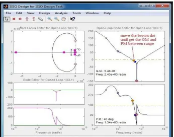
After completing the transfer function calculation, the transfer function of open loop system and closed loop system has identify. The toolbox like SISO Tool is used to obtain the controller parameter for PID controller. The PID controller is design based on the stated system by using Bode plot. The range of the phase margin is 40º to 60º and gain margin is 2dB to 6dB. For patch actuator, phase margin, Pm = 40º at frequency 214Hz.

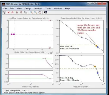
For patch actuator, gain margin Gm = 5.46 dB at frequency 387Hz and phase margin, Pm = 40º at frequency 214Hz and for bender actuator, gain margin Gm = 6.45dB at frequency 387Hz and phase margin Pm = 46.6º at frequency 184Hz. The magnitude of gain margin and phase margin are in range of stability. Figure 4.8 and Figure 4.9 shows the Bode diagram for an open loop system.

Figure 4.9: Bode Diagram for Bender Actuator in Open Loop System

A number of simulations with respects to the open loop and the close loop system characteristics of the controller are previous knowledge. An appropriate value of the PID controller is selected based on the values of the phase margin and gain margin. The simulations for of open loop system of the transfer function are plotted in Nyquist Bode diagram.

Figure 4.10: Nyquist Diagram of the Open Loop for Patch Actuator

Figure 4.11: Nyquist Diagram of the Open Loop for Bender Actuator

The close loop transfer function is defined and plot into Bode diagram. From the Bode diagram, the value of bandwidth can be determined. The magnitude frequency is approximately at -3dB.

The bandwidth for patch actuator is 471Hz at -3dB and bandwidth for bender actuator is 441Hz. The bandwidth gives the accuracy of the system performance to eliminate the error on the system. From the value of bandwidth, controller parameter to PID controller is suitable and accepted. Figure 4.12 and Figure 4.13 shows the Bode diagram for the close loop system.

Figure 4.13: Bode Diagram for Bender Actuator in Close Loop System

Table 4.3: Controller Parameter for Patch Actuator

SISO Tool

Kp (volts/µm)

Ki (volts/µm·sec)

Kd (volts·sec/µm)

Phase Margin (deg)

Gain Margin (dB)

Bandwidth (Hz)

Table 4.4: Controller Parameter for Bender Actuator

SISO Tool

Kp (volts/µm)

Ki (volts/µm·sec) Gain

Kd (volts·sec/µm)

Phase Margin (deg)

Gain Margin (dB)

4.6 Comparative Study and Discussion

The patch actuator has undergone two different types of methods to determine the controller parameter. These two different methods will give different values for the parameters. The difference of these methods is discussed in the Table 4.5 below:

Table 4.5: Patch Actuator Comparison

Heurestic SISO Tool

Kp (volts/µm) 0.99 2.068e-07

Ki (volts/µm·sec) 10000 7104

Kd (volts·sec/µm) 0.00035 5.718e-05

Phase Margin (deg) 36 40

Gain Margin (dB) 7.21 5.46

Bandwidth (Hz) 1.28 471

The value for the Kp, Kd and Ki for the SISO Tools is affected by the phase margin and the gain margin. As for the heuristic method, the phase margin and the gain margin are affected by the Kp, Ki and Kd.

Table 4.6: Bender Actuator Comparison

Heurestic SISO Tool

Kp (volts/µm) 0.05 3.289e-17

Ki (volts/µm·sec) 11 1971

Kd (volts·sec/µm) 0.00005 1.273e-22

Phase Margin (deg) 49.3 46.6

Gain Margin (dB) 9.79 6.45

Bandwidth (Hz) 520 441

The controller parameter is obtained depending on phase margin and gain margin. For the heuristic method, the controller parameter to PID controller is based on trial and error and the values refer to phase margin and the gain margin.

From the Table 4.6, SISO Tool is suitable and more accurate than the heuristic method. The PID controller parameter is achieved as expected. To determine the overshoot for the bender actuators, the setting value for the gain margin is 2dB to 6dB and required value for the phase margin is set to Pm = 46.6º. Meanwhile, the value phase margin Pm = 49.3º for heuristic method is higher than SISO Tool. The high value phase margin will lower the overshoot for the system. Thus, less error will occur by using heuristic method.

4.6 Overall Discussion

In the discussion, this section refers the previous Bode diagram and the Nyquist diagram result to validate the stability of the open loop and the closed loop system. The SISO Tool method is more accurate and obtained stable system than the heuristic method. This is because the values for phase margin are 40º to 60º and gain margin is 2dB to 6dB and the SISO Tool value is between the ranges. The effect of patch and bender is the overshoot is lower than heuristic method.

CHAPTER 5

CONCLUSION

5.1 Conclusion

In conclusion, the background of the project has discussed about the characteristic and the function for piezoelectric actuator. The problem for this piezoelectric actuator, the transfer function for the system is unstable. The PID controller will be use to control the displacement. The objective for this project is to compare and also analyze the patch and bender actuator and identify the controller parameter that use to control the unique transfer function from patch and bender actuator. The simulation from MATLAB of displacement will generate and the displacement output will be controlled with PID controller. The simulation will be simulated by MATLAB and SISO Tool software. The understanding about PID controller is required because the parameter of Ki, Kp and Kd will be determined. The advantage of use the PID controller is it can stable the system in the control system.

For the methodology, it has discuss the method that has been use to solved the problem. This problem can be solved using the heuristic method and SISO Tool. The heuristic method is the trial and error using the MATLAB software on the m.file format. The m. file is developed by the MATLAB software that use in the command window. The studies in MATLAB and software are required to solve the problem with this report. The programming is developed based on the experimental rigs that have bender and patch actuator that include the PID controller. The best method is the SISO Tool because this tool is more accurate than the heuristic method that to determine the controller parameter for PID controller.

In the result, it has show the results simulation for the open loop and close system. The controller parameter for PID controller has been obtained to control the displacement. The controller parameter is determined based on phase margin and gain margin. The range for the phase margin is 40º to 60º and the gain margin is 2dB to 6dB. There are two method approached to determined the controller parameter for PID controller. The heuristic method was determined the controller parameter using trial and error. This method was taken more time to obtain the controller parameter and also get the stability for the open loop and close loop system. The SISO Tool method is the best method to determine the controller parameter and also less time than heuristic method. The Bode diagram and Nyquist diagram show the stability for open loop and close loop system.

5.2 Future Works

5.2.1 Simulink

Simulink is the toolbox from the MATLAB software that used to simulate and also determine the controller parameter for PID controller. Simulink can add the block to control the displacement and obtained more accurate result from the previous analysis.

5.2.2 Loop Shaping System

REFERENCES

Jong-Jer Tzen, Shyr-Long Jeng and Wei Huang Chieng (2001). “Modelling of Piezoelectric Actuator for Compensation and Controller Design.” Precison Engineering. pp. 70-86

Baek-Ju Sung and Eun-Woong Lee (1987). “Displacement Control of Piezoelectric Actuator using the PID Controller and System Identification Method.” IEEE.

J. Sloss, J. Bruch, S.Adali and I.S Sadek (2001). “Piezoelectric Patch Control using an Integral Equation Approach.” Thin-Walled Structures. Vol. 39, no.1, pp. 45-63

Dunsch, R., & Breguet, J.-M. (2007). “Unified Mechanical Approach To Piezoelectric Bender Modeling.” Sensors and Actuators A: Physical, Vol. 139, no.2, pp. 436–446.

Antonio Visioli (2006). “Advances in Industrial Control.” Practical PID Control, no. 1 pp. 1-18

Novotny, M., and Ronkanen, P. (1997). “Piezoelectric Actuators.” pp. 1–12

Physik Instrumente (2008). “ Piezo Nano Positioning : Patch and Bender Actuator.” Available at: http://www.physikinstrumente.com. (Accessed date: 10 October 2012)

Norman S.Nise (2004). “Control System Engineering” California State Polytechnic University Pomona, pp. 12-13

Mathworks (2012). “PID Control with MATLAB and Simulink.” Available at:

Mizuno, Takeshi Furushima, Takehiko Ishino, Yuji Takasaki and Masaya (2007). “Application Of Displacement Cancellation Control To Vibration Isolation System”

2007 International Conference on Control, Automation and Systems, pp. 335-338

M. Chidambaram and I. Ananth (1999). “Closed-loop Identification of Transfer Function Model for Unstable Systems” The Franklin Institute, pp 1055-1061

Mohd Nazmin Maslan, M. Mailah and I.Z.M Darus (2012) “Identification and Control of A Piezoelectric Patch Actuator” Systems Science and Computational Intelligence, (Universiti Teknologi Malaysia)

APPENDICES

(MATLAB PROGRAMMING)

clc,clear;

% Patch transfer function

num =[0.03747 -0.07066 0.03319] % numerator

a = 0.4882; % denominator

b = -1.492;

c = 0.0039;

G = tf(num,[a b c]) % transfer function for patch

[num,den] = pade (0.00065,2)% time delay, second order system

delay_tf=tf(num,den) % transfer function for time delay

P = (250/100); % converter

G_delay= G*delay_tf % transfer function with time delay

V = G_delay*P % transfer function multiple with converter

% Controller Setting

Kp= 0.99; % Proportional

Ki= 10000; % Integral

Kd= 0.00035; % Derivative

% PID transfer function

s=tf('s');

PID=tf(Kp + Ki/s + Kd*s); % PID equation

% Analysis from the G(s)

% Open loop system

figure(1);margin(L); % generate the bode diagram for open loop

system

figure(2);nyquist(L); % generate the Nyquist plot

% Closed loop system

T=feedback(L,1); % declare the close loop system for the

transfer function

figure(3);bode(T); % generate for bode diagram for close loop

system

---

clc,clear;

% Bender transfer function

num =[0.211 -0.2131 0.0021] % numerator

a = 0.1348; % denominator

b = -1.13;

c = -0.0048;

G = tf(num,[a b c]) % transfer function

[num,den] = pade (0.00065,2)% time delay, second order system

delay_tf=tf(num,den) % transfer function for time delay

P = (60/160) % converter

G_delay= G*delay_tf % transfer function with time delay

V = G_delay*P % transfer function multiple with converter

% Controller setting

Kp= 0.05; % Proportional

Ki= 11; % Integral

Kd= 0.00005 % Derivative

% PID transfer function

s=tf('s');

% Analysis from the G(s)

% Open loop system

L=(PID*V);

figure(1);nyquist(L); % generate the bode diagram for open loop

system

figure(2);margin(L); % generate the Nyquist plot

% Closed loop system

T=feedback(L,1); % declare the close loop system for the

transfer function