A high precision accelerometer-based sensor unit for the acquisition of ultra low distortion seismic signals

City, University of London Institutional Repository

Citation

:

This is the accepted version of the paper.

This version of the publication may differ from the final published

version.

Permanent repository link: http://openaccess.city.ac.uk/19360/

Link to published version

:

Copyright and reuse:

City Research Online aims to make research

outputs of City, University of London available to a wider audience.

Copyright and Moral Rights remain with the author(s) and/or copyright

holders. URLs from City Research Online may be freely distributed and

linked to.

A High Precision Accelerometer-Based Sensor Unit

For the Acquisition of Ultra Low Distortion

Seismic Signals

By

Panagiotis Ioakim

A thesis submitted for the degree of

Doctor of Philosophy

July 2017

CITY

UNIVERSITY OF LONDON

~ 2 ~

Is there a more noble cause for science other than the advancement of

our profound understanding of self and our surroundings? To this end,

is there a more effective way to unravel the obstacles to such

understanding, other than to seek out the very root of their existence?

To the pillars of the past, the visionaries of the present,

~ 3 ~

Abstract

Over 800,000 people worldwide lost their lives to earthquakes in the last decade and on average 171 people die every day due to earthquake related damage to structures and buildings. Precisely understanding the effects ground motion has on manmade structures is crucial to making them earthquake resistant. This can only be achieved by the precise measurement, recording, and analysis of ground displacement trends during a seismic event.

Although there is a vast amount of recorded seismological data available, current technology and processing methods fail to represent accurate ground displacement over time as the considerable technological challenges have yet to be overcome.

Raw seismic data has so far been primarily acquired with instruments utilising geophone or accelerometer based sensors. These instruments produce prominent time domain displacement errors due to the various system and sensor inaccuracies, and due to non-linear response. Since accelerometers provide acceleration over time data: whilst geophones are velocimeters, and therefore provide velocity over time data; in order to derive true ground displacement over time, a double, or single numerical integration is required respectively. During this essential numerical integration processes of data from such sensors, even small in magnitude errors accumulate to yield rather large displacement trend offsets over a typical event recording period of 60 to 120 seconds. In addition, the numerical integration process itself poses considerable challenges due to the theoretically infinite number of samples and the accurate determination of initial conditions required for an exact mathematical result to be obtained. The latter, is currently performed by averaging an up to 60 second pre-event data trend stored on the instrument.

~ 4 ~

accuracy of the initial assumptions made about a specific set of data. Faced with such a multivariable and uncertain dynamic behaviour, where even mathematical system modelling is of inadequate long term accuracy, a solution that aims to directly minimise these errors at source, rather than attempt to correct them post-acquisition, is of immense importance when it comes to the recording, analysis, and understanding of earthquakes.

~ 5 ~

Acknowledgements

I would like to thank all those who have directly and indirectly helped make this work possible. In particular, I would like to thank my parents for their unconditional and continual support, and their tireless encouragement throughout the years.

A special thanks to my wonderful partner Jenny for her unwavering faith, support, and trust in me and my work, during the good, and during the difficult times. Thank you for being such a fantastic and positive influence in life.

My children Sophia and Helena, who have shown great understanding of my frequent absence of mind; Lottie and Sally, who have grown to sympathise with the amount of work such an undertaking requires, and everyone’s kind moral support.

My good friend and fellow engineer Mr Enyi Ogbuehi, for acting as my sounding board for even the most off-the-wall ideas.

I would like to thank Dr Andrew Chanerley for introducing me to the exciting field of seismic instrumentation, and the numerous members of staff at the University of East London for their support.

The staff at City University of London: Professor Nicholas Karcanias for his most welcoming attitude towards my research project, Professor Panos Liatsis for all his advice and research support which lead to my research fellowship at the university, Dr Stathis Milonidis for his support in the role as my second supervisor, and of course, I would like express my greatest gratitude to my exceptional supervisor and now friend Dr Iasonas Triantis, for his excellent moral support, his outstanding academic mentoring, and his extraordinary efforts beyond expectation to guide me to the successful completion of this work. I thank you.

~ 6 ~

Table of contents

Abstract 3

Acknowledgements 5

List of figures and tables 10

Glossary of terms 15

1. Introduction 16

1.1 Preface 16

1.2 Inherent seismic sensor limitations 23

1.3 The need for an improved seismic sensor 26

1.4 Motivation and project aims 28

1.5 Novelty and contribution to knowledge 29

1.6 Thesis organisation 30

1.7 List of publications 31

2. Principles of seismic data acquisition 32

2.1 Introduction to Seismology 32

2.1.1 Seismic Waves 33

2.1.2 The Earth’s structure 36

2.1.3 Early seismographs 37

2.2 Modern seismographs 51

2.2.1 Geophones 52

2.2.2 MEMS Accelerometers 52

2.2.3 Signal conditioning 60

2.2.4 Signal conversion and storage 62

2.3 Post digitisation processing 65

2.3.1 Digital filtering 65

2.3.2 Numerical integration 66

2.4Conclusion 67

3. Non ideal instrument functionality 70

3.1 Evaluation of the MEMS accelerometer sensor performance 84

3.1.1 MEMS Sensor noise experimental investigation 88

3.1.1.1 Experimental investigation of temperature effects on sensor noise 91

3.1.1.2 Experimental investigation of differential Bi-axial excitation for

noise reduction 94

3.1.1.3 Conclusion on sensor noise investigation 96

~ 7 ~

3.1.2.1 Sensor Frequency response acquisition via electrostatic frequency-sweep

97

3.1.2.2 Sensor output dithering via high frequency electrostatic excitation 98

3.1.2.3 Sensor dynamic response acquisition via electrostatic impulse

excitation 100

3.1.2.4 Sensor phase response determination via frequency-sweep excitation

102

3.1.2.5 Sensor on-demand dynamic response determination conclusion 104

3.1.3 Experimental investigation of non-linear sensor response 105

3.1.3.1 Experimental investigation of potential sensor hysteretic behaviour

105

3.1.3.2 Experimental investigation of sensor cross-axis interference 108

3.1.3.3 Cross Axis interference theory development and experimental verification

112

3.1.3.4 Sensor Cross Axis interference conclusion 118

3.1.4 Temperature related errors 118

3.1.4.1 Temperature related errors conclusion 119

3.1.5 Investigation of fabrication based errors 119

3.1.5.1 Fabrication based errors conclusion 120

3.2 Analytical evaluation of front end electronics 121

3.2.1 Filter phase and attenuation investigation 121

3.2.1.1 Filter phase and attenuation conclusion 122

3.2.2 Investigation of offsets and drifts in the front end electronics 123

3.2.2.1 Investigation of offsets and drifts in the front end conclusion 124

3.3Evaluation of digitisation errors 124

3.3.1 The Quality Preservation Sampling (QPS) criterion 126

3.4 Soil dynamic effects 127

3.4.1 Dynamic and static tilts 127

3.4.1.1 Dynamic and static tilts conclusion 130

3.5Conclusion 132

4. Realisation of the HPAGS sensor 135

4.1 Electronic Systems 136

4.2 The physical layout 150

4.3 The electromechanical assembly 151

4.3.1 The gyro stabilisation system 152

4.3.2 The power commutation system 154

~ 8 ~

4.4 Control and embedded software 157

4.4.1 PC Host Instrument Control Software 157

4.4.2 Embedded Software 159

5. HPAGS Tests and results 161

5.1 Sensor calibration process 161

5.2 FIR Low-Pass 100Hz Filter design 165

5.3 Setting the assessment standards 166

5.4 HPAGS auto-zero bias correction assessment. 170

5.4.1 Results 171

5.4.2 Conclusion 175

5.5 Input re-composition by impulse de-convolution 176

5.5.1 Results 176

5.5.2 Conclusion 181

5.6 HPAGS gain error correction assessment 182

5.6.1 Results 182

5.6.2 Conclusion 183

5.7 HPAGS cross-axis sensitivity correction assessment 184

5.7.1 Results 184

5.7.2 Conclusion 186

5.8 HPAGS gyro stabilisation module assessment 187

5.8.1 Static evaluation of gyro motor noise 187 5.8.2 HPAGS active gyro correction assessment 189

5.8.3 Results 193

5.8.4 Conclusion 200

6. Conclusion 201

7. Future work 205

References 206

Appendices

Appendix A- Windows control software 216

Appendix B- Embedded software 220

Appendix C- Matlab function script 228

~ 9 ~

I hereby certify as the author, that to the best of my knowledge, the

content of this thesis is exclusively my own work, and that any inclusions

and references to other work have been appropriately acknowledged.

~ 10 ~

List of figures and tables

Chapter 1

Figure 1 Pescara del Tronto earthquake, central Italy, 2016. (Source: REUTERS/Adamo

Di Loreto) 16

Figure 1.1 Tectonic plate faults. (a) Normal fault. (b) Reverse fault. (c) Strike-slip fault 17

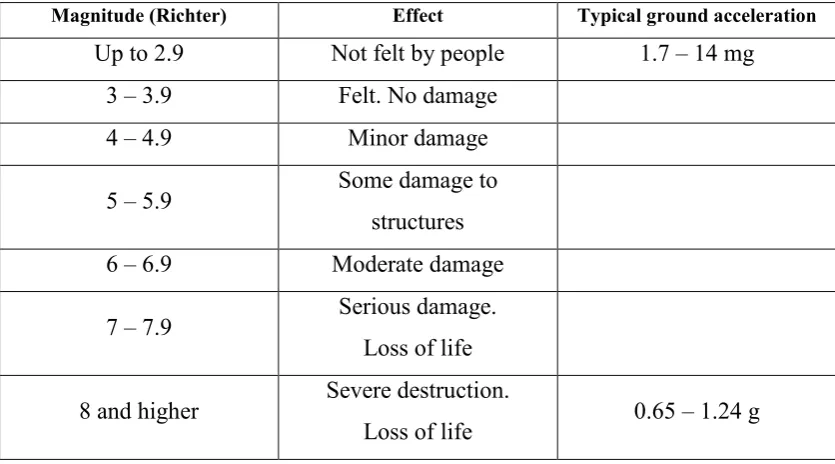
Table 1 The Richter scale of earthquake magnitude 18

Figure 1.2 Baseline spline correction example. (Source public domain) 20 Figure 1.3 Acceleration without rotational component (a), and with rotational _{component (b).} 21

Figure 1.4 Non sensor concentric rotation due to acceleration. 21

Figure 1.5 Frequency response of a typical GS11D geophone by Geospace _{Technologies.} 23

Figure 1.6 Measured frequency spectrum of unfiltered MEMS accelerometer. 24

Figure 1.7 Exemplification of baseline error [22]. 27

Chapter 2

Figure 2 The propagation of a compression wave 33

Figure 2.1 The propagation of a shear wave 34

Figure 2.2 Ground roll motion of Rayleigh waves 35

Figure 2.3 A typical seismograph record of one axis 35

Figure 2.4 Earth’s structure 36

Figure 2.5 Typical mass-spring arrangement 38

Figure 2.6 Second order system response to a step function at various damping rates 41

Figure 2.7 Natural resonance of systems 42

Figure 2.8 Phase response of systems 43

Figure 2.9 Velocimeter arrangement 44

Figure 2.10 Frequency, velocity and acceleration responses of_{(B) Velocity Sensor: (C) Acceleration Sensor} (A) Mechanical Sensor: 45

Figure 2.11 The “Garden gate” arrangement 46

Figure 2.12 Inverted pendulum arrangement 47

Figure 2.13 The “LACoste” seismometer arrangement 48

Figure 2.14 Force balance sensor employing closed loop compensation 50

Table 2 Earth bandwidth of interest 51

Figure 2.15 A typical Geophone arrangement 52

Figure 2.16 An illustrational view of a MEMS accelerometer’s internal structure 53 Figure 2.17 Anti-phase excitation of differential capacitance structure 54

Figure 2.18 Synchronous demodulator 58

Figure 2.19 Lock-in amplifier utilising square wave modulation 59

Figure 2.20 A typical data acquisition system 60

Figure 2.21 Unique elaborate seismograph front end 61

~ 11 ~

Figure 2.23 Acceleration trends of (a) El Centro, (b) Northridge, and (c) Llolleo _earthquakes 64

Figure 2.24 Typical system installation 68

Figure 2.25 A typical self contained seismograph 68

Table 2.1 Technical characteristics of a modern seismograph 69

Chapter 3

Figure 3 Block diagram of sensor to displacement data process 70

Figure 3.1 The primary MEMS test platform 73

Figure 3.2 Photocurrent to voltage convertor circuit 74 Figure 3.3 Non-contact range finder optics arrangement 75 Table 3 Non-contact range finder output, derivative and inverse square curve fit 75 Figure 3.4 Voltage to distance characteristic of the non-contact range finder 76

Figure 3.5 Dynamic response of the non-contact rangefinder monitoring the vibration of _{a leaf spring} 76

Figure 3.6 Optical encoder induced rangefinder output 77

Figure 3.7 The mechanical vibration platform 78

Figure 3.8 First Primary MEMS platform raw vibration results 79 Figure 3.9 Compact assembly directly bonded to the shaft 79 Figure 3.10 Resin bonded compact assembly output with improved noise characteristics 80 Figure 3.11 Digitised and mathematically zero-g offset corrected raw accelerometer data 81 Figure 3.12 First integral of the raw data representing velocity over time 81

Figure 3.13 Second integral of the raw data representing displacement over time, _{exhibiting baseline offset error} 82

Figure 3.14 Acceleration data, first and second integrals of filtered and AC coupled _sensor 83

Figure 3.15 Prominent sources of potential error identified by section 84 Figure 3.16 Diagrammatic representation of the ADXL327 sensor 87

Figure 3.17 Sensor noise frequency spectrum 88

Figure 3.18 Circuit diagram of sensor noise investigation circuit 91 Figure 3.19 Physical assembly of sensor noise investigation circuit 91 Figure 3.20 direct sensor output at rest and at different temperatures 92 Table 3.1 Statistical analysis of the output trends of Figure 3.20 92 Figure 3.21 Standard deviation of sensor noise over temperature 93

Figure 3.22 Noise range over temperature 93

Figure 3.23 x-axis sensor output at no excitation 94

Figure 3.24 y-axis sensor output at no excitation 94

Figure 3.25 Differential excitation of sensor axis 95

Figure 3.26 x and y axis output segment comparison 95

~ 12 ~

Figure 3.30 Sensor impulse response via the use of the test pin 101

Figure 3.31 Integral of sensor impulse response 102

Figure 3.32 Sensor phase response derived via test pin excitation 103 Figure 3.33 Sensor phase response magnified segment 104

Figure 3.34 Mechanical rotational platform 105

Figure 3.35 Sensor on rotational platform a initial position 106 Figure 3.36 y-axis voltage output for 0 - 180 rotation and back to zero 107 Figure 3.37 y-axis voltage output for 0 - 3600 rotation and back to zero 107 Figure 3.38 Folded y-axis output along the 180 line 108 Figure 3.39 Experimentally derivedy-axis output with respect to g 108 Figure 3.40 Expected calculated output of y-axis over a 0 - 360 rotation and back 109 Figure 3.41 Calculated output of y axis with the added z-axis 1% cross-axis contribution 110 Figure 3.42 Mathematically derived y-axis output compared with experimental results 111 Figure 3.43 Mathematically derived y-axis output with added 2% cross-axial sensitivity 112 Figure 3.44 SlicedMEMS IC under microscope showing corner spring structure 112

Figure 3.45 Sliced_structureMEMS IC under microscope showing inertial mass suspension 113

Figure 3.46 Diagrammatic arrangement of inertial mass suspension 113 Figure 3.47 Inertial mass displacement vector due to uneven spring compression 114 Figure 3.48 Inertial mass displacement vector due to uneven spring tension 114 Figure 3.49 Mathematically corrected experimental y-axis output using equation 3.22 116

Figure 3.50 Voltage output over temperature 118

Figure 3.51 MEMS package to silicon die misalignment 120

Figure 3.52 RC filter amplitude over frequency characteristic 122 Figure 3.53 Sampled signal exhibiting digitisation errors 125

Figure 3.54 Rotation of obelisk after the 1897 Great Shillong Earthquake (Source: Report _{on the Great Earthquake of 12}th_{June 1897.Mem. Geol. Survey India, vol. 29.}

(from figure 1)).

128

Figure 3.55 Vertically misaligned sensor 129

Figure 3.56 Gradients around 0 ofSine and Cosine graphs 130

Figure 3.57 Sensor near underground boundary 131

Chapter 4

Figure 4 Specification diagram of HPAGS sensor base on error analysis 135

Figure 4.1 HPAGS system level diagram 136

Figure 4.2 HPAGS circuit with only one out of the three channels depicted 140

Figure 4.3 Detail of MEMS circuit 141

Figure 4.4 HPAGS sensor power supply and precision reference circuit detail 142 Figure 4.5 MEMS sensitivity drift due to supply voltage change 143

Figure 4.6 Active filter circuit detail 144

~ 13 ~

Figure 4.8 Amplitude comparison between HPAGS and current state of the art _{instrument filters} 146 Figure 4.9 Auto-zero correction feedback loop detail 147

Figure 4.10 Action of HPAGS sensor’s Auto-Zero correction circuit and algorithm 148 Figure 4.11 Impulse response of x-channel derived by electrostatic excitation 149 Figure 4.12 HPAGS sensor’s electronics physical layout 150 Figure 4.13 The Active Gyro-Stabilised electromechanical assembly 151

Figure 4.14 Gyro assembly detail 153

Figure 4.15 Through-bearing power commutation detail 154 Figure 4.16 Assembled bearing and commutator detail 155

Figure 4.17 Six degrees of freedom gimbal assembly 156

Figure 4.18 Bespoke Windows based host instrument control software 157 Figure 4.19 HPAGS sensor embedded software flowchart 159

Chapter 5

Figure 5 Spatial orientations for calibration 161

Figure 5.1 High accuracy rotational platform 162

Figure 5.2 Kaiser Window amplitude response (fc=100Hz, fp=102 Hz) 165 Figure 5.3 Kaiser Window phase response (fc=100Hz, fp=102 Hz) 166 Figure 5.4 Kaiser Window impulse response ( fc=100Hz, fp=102 Hz) 166

Figure 5.5 Mechanical vibration platform with HPAGS electronics affixed to the

excitation shaft 169

Figure 5.6 _{Unfiltered IR displacement sensor data} 170

Figure 5.7 Auto-zero versus conventionally average-subtraction corrected acceleration

trends 171

Figure 5.8 Auto-zero, and conventionally corrected best-fit linear displacement trends 172 Figure 5.9 Auto-zero bias correction system block diagram 172

Figure 5.10 Voltage at ADC input 173

Figure 5.11 Means ofConventionally, HPAGS, and HPAGS improved bias corrected

signals 174

Figure 5.12 Displacementbest-fit lines ofConventionally, HPAGS, and HPAGS

improved corrected signals 174

Figure 5.13 Auto-zero corrected and filtered acceleration trend 176 Figure 5.14 Electrostatically triggeredImpulse response 177

Figure 5.15 Impulse response of x-axis channel 177

Figure 5.16 _{Frequency spectrum of x-axis impulse response} 178 Figure 5.17 Frequency spectrum of HPAGS x-axis output. 178

Figure 5.18 Frequency spectrum of the division of the acceleration and impulse response

spectra 179

~ 14 ~

Figure 5.21 Synthesised high frequency input 180

Figure 5.22 Evaluated output by convolution of high frequency inputand Impulse

response 181

Figure 5.23 Outputdifference between expected and gain-corrected trends 183

Figure 5.24 Acceleration trend of x-axis output 184

Figure 5.25 Acceleration trend of y-axis output 185

Figure 5.26 Comparison between x-axis raw, cross-axis corrected, and y-axis data 186 Figure 5.27 x-axis displacement data; uncorrected, and cross-axis corrected 187 Figure 5.28 _{HPAGS x-axis output with vertical gyros on.} 188 Figure 5.29 _{Frequency spectrum of the HPAGS x-axis output with vertical gyros on.} 188

Figure 5.30 Spectrum comparison between unfiltered (blue) and filtered sensor outputs

(red). 189

Figure 5.31 TheHPAGS sensor attached onto the CNC machine 190 Figure 5.32 HPAGS sensor attachment to the CNC bed detail 191 Figure 5.33 HPAGS sensor on CNC bed top view diagram 192 Figure 5.34 HPAGS x and y-axis acceleration data of machine bed 193 Figure 5.35 HPAGS x and y-axis velocity data of machine bed 194 Figure 5.36 HPAGS x and y-axis displacement data of machine bed 194 Figure 5.37 HPAGS x and y-axis acceleration data in rigid mode. 195 Figure 5.38 HPAGS x and y-axis velocity data in rigid mode. 195 Figure 5.39 HPAGS x and y-axis displacement data in rigid mode. 196

Figure 5.40 HPAGS motion in rigid mode. 196

Figure 5.41 HPAGS x and y-axis acceleration data in gyro mode. 197 Figure 5.42 HPAGS x and y-axis velocity data in gyro mode. 198 Figure 5.43 HPAGS x and y-axis displacement data in gyro mode. 198

Figure 5.44 HPAGS sensor’s motion in gyro mode. 199

~ 15 ~

Glossary of terms

1/f noise Noise with a power spectral density inversely proportional to its frequency

Accelerometer A device that measures acceleration ( rate of change of velocity)

Belt (seismic) A narrow geographic zone on the surface of the Earth along which _{earthquake activity occurs.}

Brownian motion Random motion of particles resulting from their collision with fast-moving atoms _{or molecules in the medium}

Brownian noise Signal noise produced by Brownian motion, also known as thermomechanical

Convolution A mathematical operation on two functions resulting in another function

Critical damping Damping which enables the system to attain steady state at the shortest time _{without oscillations} Cross-axis

sensitivity The amount of output that is observed on the sensing axis stemming from accelerations on a perpendicular axis

Damping The reduction in amplitude of an oscillation by frictional or other resistive forces

Damping coefficient The ratio of damping to critical damping.

Decimation The process of reducing the sampling rate of a signal

De-convolution The inverse of convolution. See convolution

Elastic propagation The propagation of waves through solid (elastic) matter

Epicentre The point on the Earth's surface that is directly above the point of origin of an _earthquake

Fault A fracture along which the blocks of Earth's crust on either side have moved _{relative to one another} Gain Bandwidth

product

The product of an amplifier's bandwidth and gain at which the bandwidth is measured

Geophone A device that converts ground movement (velocity) into voltage utilising a _{moving magnet within a coil}

Ground tilt The deviation of the ground from what is accepted to be horizontal during an _earthquake

Homogeneous fluid A fluid that has the same proportions of its components throughout a given _{sample, thus uniform in composition}

HPAGS Sensor High Precision Active Gyro-Stabilised Sensor

Hypocentre The point within the Earth where an earthquake rupture starts

Least squares regression

A statistical method used to determine a line of best fit by minimizing the sum of squares created by a mathematical function

Long period instrument

An instrument in which the resonant frequency is very low, usually designed for seismic signals in the range 1 Hz to 10 Hz

Mantle The part of the Earth between the core and the crust

MEMS Sensors Miniature sensors incorporating mechanical structures and electronic circuits

Micromachining The technique for fabrication of structures on the micrometer scale

Near-field

Earthquake An earthquake which occurs close to the fault. See fault

Piezoelectric effect The ability of certain materials to generate a voltage when subjected to _{mechanical stress or vibration}

Piezoresistive effect A change in the electrical resistivity of a material when mechanical stress is _applied

Polysilicon A high purity, polycrystalline form of silicon

RS232 A standard for serial communication transmission of data

Short period instrument

An instrument in which the resonant frequency is high, usually designed for seismic signals in the range 0.01 Hz to 0.1 Hz

Slew Rate The maximum rate at which a system can respond to an abrupt change of input

Spline A mathematical function defined piecewise by polynomials

Subduction zone A point at which one tectonic plate is forced underneath another

Tectonic plates Sub-layers of the Earth's crust that move independently over the mantle

~ 16 ~

Chapter 1

Introduction

Earthquake: A sudden violent shaking of the ground, typically causing great destruction, as a result of movements within the earth's crust or volcanic action.

(Oxford dictionary)

1.1 Preface

Nearly fifty thousand noticeable earthquakes occur every year on Earth, out of which one hundred are capable of - often devastating - damage to buildings. Over the recorded history of mankind, earthquakes have been responsible for the deaths of millions of people and the destruction of entire cities.

Figure 1 Pescara del Tronto earthquake, central Italy, 2016. (Source: REUTERS/Adamo Di Loreto)

~ 17 ~

Tectonic earthquakes are the result of sudden relative movement of the Earth’s surface plates. As these plates are in continuous motion, anomalies on their boundaries tend to cause localised frictional resistance, resulting in a large build up of energy. Stresses exceeding the natural strength of the retaining material, inevitably cause a sudden release of energy which manifests itself as a fracture or slip that can extend to several kilometres. The relative ground movement caused by these fractures is usually small, however on occasion tectonic movements will generate major earthquakes such as the 1906 San Andreas Fault event, where the ground was displaced horizontally by nearly 6 meters.

Figure 1.1 Tectonic plate faults. (a) Normal fault. (b) Reverse fault. (c) Strike-slip fault

Tectonic plate movement can manifest itself in different ways, all capable of causing large magnitude earthquakes: It can be vertical in nature, where one plate sinks with respect to the other, or rises due lateral compressive forces, or it can be horizontal, where the two plates slip past each other in a coplanar fashion.

Due to the considerable variation in seismic motion over an area, the effects of a seismic event can be difficult to directly quantify, hence qualitative scales of

intensity have been used since the late 19th century. It wasn’t until the development of seismographs that magnitude became a quantitative measure of the amplitude of seismic waves generated by an earthquake. In 1935 Charles F. Richter introduced his logarithmic Richter scale of magnitude, which was based on the amplitude recorded on a standard for the epoch seismometer, at a 100 Km distance from the

(a) (b)

~ 18 ~

epicentre. Table 1 depicts the effects caused by an earthquake according to the Richter scale magnitudes.

Magnitude (Richter) Effect Typical ground acceleration

Up to 2.9 Not felt by people 1.7 – 14 mg 3 – 3.9 Felt. No damage

4 – 4.9 Minor damage

5 – 5.9 Some damage to structures 6 – 6.9 Moderate damage

7 – 7.9 Serious damage. Loss of life

8 and higher Severe destruction.

Loss of life 0.65 – 1.24 g

Table 1 The Richter scale of earthquake magnitude

Seismographs are by default inertial systems and therefore their outputs are generally accelerometric. One exception is the geophone sensor, which converts the inertial motion into an electrical signal by means of a magnet within a moving coil, thus able to provide a direct velocimetric output. The conversion therefore of a signal acquired by a seismograph necessitates the single or double integration of the data depending on the sensor used in order to acquire a ground displacement over time trend. The cumulative effects of the integration process hugely exaggerate any errors in the data, and in combination with systematic errors, render earthquake data inaccurate to a degree which greatly affects our understanding of them and inevitably our efforts to better protect structures from their devastating effects.

~ 19 ~

Recent technological developments such as micromachining, precision low noise integrated circuits, and encapsulation techniques, have vastly improved the stability and operation of seismometers, however, due to many inherent physical and electronic limitations, much improvement is still necessary if such instruments are to yield useful near-true to the original earthquake displacement over time data.

A vast amount of more recent seismological data exists that has been acquired primarily with instruments utilising geophones and accelerometers since the 1960s. Since these instruments employ the aforementioned velocimetric or accelerometric sensors, time domain displacement data can only be acquired after one or two numerical integration processes respectively. The data acquired from such instruments inevitably contains cumulative integration errors resulting from various inaccuracies within the instrument, which together conspire to produce rather large errors in the displacement data trends, termed baseline offset.

It is not atypical for a seismic data displacement trend to show after-event displacement errors in the region of several meters, whilst in reality the end ground displacement has indeed been zero. These inaccuracies are predominately caused by the instrument’s electronics practical limitations, but also due to internal to the sensor non-linearities, noise, and drifts, requiring rather involved calibration processes [1][2] [3] [4].

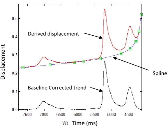
Current data processing methodologies necessitate the use of post-digitisation algorithms to reverse such displacement errors once the true end displacement is made known, usually via the Global Positioning System (GPS). By knowing the true end displacement of the trend, and assuming a zero averaged initial condition, a spline baseline correction can be imposed as shown in figure 1.

~ 20 ~

Figure 1.2 Baseline spline correction example. (public domain)

Whilst these methods produce workable results, some necessitate the use of accurate GPS instrumentation with long term data averaging in order for precise end-displacement values to be acquired. More importantly, most methods assume a progressive and mathematically predictable ground motion, where in reality the true ground displacement can easily be masked within the usually exponential in nature baseline offset.

In addition to instrument based errors, external factors, other than temperature fluctuations, can also significantly interfere with the accurate acquisition of seismic data. Ground tilts and dynamic rotations occurring during strong near-field earthquakes have been shown to have a considerable effect on seismic instruments and therefore on the data derived by these [6], [7]. Although at first, correcting for such tilts and rotations may appear easily accomplishable, the fact that the centre of such rotations is not only unknown but also variable poses a rather difficult problem to solve.

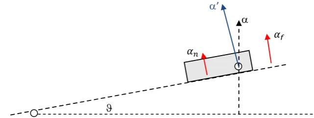
It has been suggested that multi-sensor instruments could resolve rotational and translational motions simply by measuring the accelerations due to tilt motion of the instrument. Although this is theoretically possible, most methods conveniently assume a body-centric model (figure 1.3).

Time (ms)

D

isp

lace

m

ent

Spline Derived displacement

~ 21 ~

Figure 1.3 Acceleration without rotational component (a), and with rotational component (b).

Figure 1.3(a) depicts the current use of sensors in the field, assuming a linear acceleration about the centre of the sensor (z-axis only shown here for clarity, but this holds true for all three axis x, y, and z). Current theory suggests that by utilising more sensors, such as accelerometers located at the periphery of the sensing instrument, differential accelerations marked as in figure 1.3(b), would be detectable and therefore such motion could be mathematically describable. In real environments however, the rotational centre locations are unknown and are not body-centric. Assuming a centre of rotation a short distance away from the sensor, as shown in figure 1.4, one could argue that the acceleration difference between the resulting acceleration vectors and could indeed be used to estimate the rotational centre and therefore help describe the motion of the body in question. In practice however, this model does not scale up since as the centre of rotation moves further away from the body of the instrument, the smaller the acceleration differential between and becomes, and therefore only a matter of a short distance before this difference is within the noise floor of the instrument.

Figure 1.4 Non sensor-concentric rotation due to acceleration.

The data corrupting effect of such tilts is of course due to the angular deviation of the sensing axis of the instrument with respect to the original frame of reference in

 ’ 



(a) (b)





~ 22 ~

all three dimensions. In this case, the true vertical acceleration  of the ground would be incorrectly measured as ’ due to the angular displacement of the z sensing axis, where . Further, due to the rotational forces, radial accelerations will also manifest themselves as additional components on the other sensing axis, making the derivation of true motion a rather impossible task.

Seismological instruments in use to date do not have adequate, if any at all, correction abilities to address the above sources of error. Furthermore, although the necessity of recording seismic signals down to DC level has been recognised for many decades [8], due to the difficulties involved with the double integration process and initial conditions determination, some seismographs employ a High-Pass filter with a low -3dB cut off frequency of 0.1Hz or below, further adding to the distortion of the low frequency seismic waves [9].

Other effects, such as long term instrument inaccuracies due to component variations over time that can considerably add to the aforementioned errors, have also been ignored by seismic instrument manufacturers. In conclusion therefore, historic seismic records to date can be considered only as approximations to the original time domain seismic waves, since the data stored and processed is distorted in amplitude, phase, and sensitivity, resulting in displacement trends containing errors, sometimes in the order of several meters.

The complexity and magnitude of these errors pose a serious problem to the worldwide seismological societies attempting to analyse and understand the underlying mechanisms of earthquakes, and to those attempting to construct earthquake resistant structures.

~ 23 ~

1.2 Inherent seismic sensor limitations

Modern inertial seismometers, of any physical scale, convert the motion of a point on the Earth’s surface to a usable electrical signal, usually utilising a suspended inertial mass. This very principle of operation limits and distorts the true ground motion signal since the inertial mass requires to be kept in place via mechanical or electromagnetic means. Such instruments inadvertently result in an output which is dependent not only on the amplitude but also the rate of change of the input signal, therefore imposing a kind of mechanical filtering to the signal of interest.

Figure 1.5 below depicts the frequency response of a popular geophone. Geophones, although also based on the inescapable inertial mass-spring setup, unlike accelerometers, produce an output proportional to velocity rather than acceleration. The electromechanical arrangement is either a suspended moving coil arround a magnet or vice versa, resulting in a driven harmonic oscillator with an electromagnetically induced output voltage: where x is the displacement of the coil with reference to the magnet.

Figure 1.5 Frequency response of a typical GS11D geophone by Geospace Technologies.

The output response of a typical geophone shown in figure 1.5 clearly indicates that although traditional geophones require a single integration in order to derive displacement data, even with corrective shunt resistors employed, their poor low frequency response deems them unusable for frequencies below 10Hz.

Shunt Resistance

A Open circuit

B 47K5 

C 18K2 

Damping

A 35%

B 50%

C 70%

A B

C

Frequency (Hz)

Outp

u

t

~ 24 ~

Micro Electro-Mechanical Sensors (MEMS) provide considerable improvement on resonance and sensitivity. The imperfect capacitance characteristics and mechanical limitations of the frequently used differential capacitance measurement mechanism however, tend to distort the signal. Inevitably, the driving electronics of the differential capacitance mechanism require an out of phase clock to be presented to the capacitor plates, which although rectified and filtered, is still present in the output signal. In addition, due to the small scale of the micro-machined inertial mass and polysilicon (Polycrystalline Silicon) springs, MEMS sensors suffer not only from Brownian and 1/f noise, but also from thermomechanical noise due to molecular agitation of the micro-scale inertial mass.

Figure 1.6 depicts the frequency spectrum of a typical unfiltered MEMS sensor output, showing both an 1/f characteristic and a near 50KHz internal clock feed-through.

Figure 1.6 Measured frequency spectrum of unfiltered MEMS accelerometer.

The physical constraints of such sensors along with the typical properties of systems on silicon further affect the response of such sensors yielding output non-linearity [10], temperature dependent effects on sensitivity [11], and various bias and cross-axis sensitivity related errors [12]. Even devices employing optical and mechanical-optical arrangements still suffer from these inherent errors due to the inescapable nature of the electromechanical arrangement [13] [14].

-130 -120 -110 -100 -90 -80 -70 -60 -50 -40 -30 -20 -10 0

0 10000 20000 30000 40000 50000 60000 70000

A

m

p

litu

d

e

(d

B

)

~ 25 ~

The necessary interfacing electronics are also subject to noise, drifts, and offsets, and the Analogue to Digital Conversion (ADC) process itself adds to the distortion of the original signal.

~ 26 ~

1.3 The need for an improved seismic sensor

The difficulty of precise seismic data recovery is of course due to the problem that a clear separation of the observer from the phenomenon observed cannot be readily accomplished, since the observer in this case is part of, resting on, the object of observation, namely the Earth. This has led to errors in the understanding of the behaviour of seismic waves which have in turn manifested themselves into instrument designs anticipating to measure such erroneous behaviour. One major such assumption has led to the design of only linear acceleration seismographs to this date, although dynamic ground tilts and rotations were observed and found to be of a large enough magnitude to distort the seismic data some decades ago. It is also becoming more evident that not only acute dynamic tilts are of importance during strong motion recordings, but post-event displacements and asymmetrical soil dynamics too can corrupt and impose hysteretic characteristics on the seismic data, as can very low frequency ground undulations. [17]

Many of the above sources of error conspire to give rise to the by far the most prominent observable effect of data corruption in the time domain, even with modern instruments; the “runaway effect” or “Baseline Error”. This most frequently encountered error is characterised by erroneous linear velocity and exponential ground displacement trend offsets, derived from the original raw acceleration data via a numerical integration process. This baseline error completely invalidates the derived velocity and displacement trends, as assumptions to its nature are made in order to secure an artificial baseline of zero offset error. This is usually accomplished by the enforcement of a corrective spline to the derived data.

Various other methods including advanced calibration and DSP techniques such as Wavelet transformation, filtering, and post-digitisation and integration corrections, have all been, and still are, employed in an attempt to reconstruct a true seismic displacement trend. [18] [19] [20] [21]

~ 27 ~

characteristic gradient, inevitably resulting in a rather large quadratic in nature displacement error after the second integration.

Figure 1.7 Exemplification of baseline error [22].

It should be noted that the above trends are only of 3s in length, however in practical earthquake studies, seismic trends are normally 60s – 120s in length, resulting in much larger cumulative displacement errors in the order of several meters.

Although modern seismographs have much improved over that last decade, acceleration data derived from these is still at best difficult to work with, and at worst so erroneous, that its usefulness as a tool for the study and understanding of earthquakes can be considered at times very limited.

~ 28 ~

dynamic in nature. Such treatment of the effects rather than the causes tends to fail to produce consistent long term results in the complexity of real environments.

Further to the inherent electronic sources of error, mechanical constraints produce their own set of challenges when it comes to acquiring uncorrupted data, which are deeply rooted within the very construction of these instruments and their environment. Efforts to model or correct for these errors has proven of limited use due to the complexity of the real dynamic environment, where excitation is not only of linear, but also of rotational nature [27] [28] [29] [30] [31] [32] [33] [34], and the soil substrate is rarely a uniform and known quantity, therefore contributing its own asymmetrical and non-linear effects on the instrument [35].

Although it is essential to understand and attempt to correct the perceivable instrument errors [36] [37] [38] [39] [40] [41] [42], a close and in depth examination of the very sources of these errors is crucial in deriving robust solutions able to provide effective long term correction within real dynamic environments.

It is only by addressing the root of these problems rather than alleviating the symptoms, that an instrument able to recover long term accurate displacement seismic data can be constructed.

1.4 Motivation and project aims

~ 29 ~

it became obvious that resolving the tilt problems alone would not yield any substantial improvement on the resulting data: The very significant contribution of the many overseen sensor and instrumentation error sources had to be predominantly addressed.

The objective of this work therefore is to research the multiple sources of error, internal to the instrument and external, and derive realisable solutions with the aim to create a High Precision Active Gyro-Stabilised (HPAGS) seismic sensor. The resulting six-degree-of-freedom MEMS-based seismic sensor should conceptually and experimentally prove beyond doubt, that the acquisition of highly accurate ground displacement data from accelerometric sensors is indeed a realisable possibility.

1.5 Novelty and contribution to knowledge

The majority of the content in Chapter 3 predominantly presents original theory and empirical evaluation of several novel methods and algorithms concerned with the correction or minimization of errors in current seismic sensing instruments. In particular: the method for the derivation of the dynamic response of a MEMS sensor, the direct generation of sensor signal dithering, the quality preservation sampling criterion, and the cross-axis sensitivity correction formulae, are all – to the author’s knowledge – both novel and a positive contribution to existing knowledge.

The realisation and experimental evaluation of the first six degree of freedom seismic sensor unit in Chapters 4 and 5, able to addresses the majority of the known and newly discovered via this research issues, also presents novel work which aims to inform the scientific society. Further, the auto-zero bias correction, and the auto gain correction circuits, along with their corresponding embedded algorithms, offer novel applications to classical feedback control and circuit theory.

~ 30 ~

1.6 Thesis organisation

The rest of the work presented herein is organised as follows:

Chapter 2 presents an introduction to seismology and seismic waves along with the structure of the Earth in order to facilitate a basic understanding of the object of interest. It then continues with a review of seismic sensors starting with the early innovations of the recent past and onto the modern day accelerometers, analysing and discussing each with respect to their features and limitations. Sections on data acquisition, digitisation, and post-processing are also included in this chapter in order to give the reader a wider view of the current methods and technology employed in the acquisition of seismic data, from the sensor in the field, to the familiar trends on the computer screen.

Chapter 3 is partly dedicated to the description of a primary study which aims to experimentally demonstrate the magnitude of the problem regarding the baseline offset effect, and then proceeds with attempts to eliminate each of the primary sources of this error, by experimentally testing novel correction hypotheses and methodologies. The work in this chapter is presented in a logical signal progression manner: from the sensor, via the front-end electronics, to the digitising circuits.

Chapter 4 presents the physical design of the unified sensor electronics and mechanical components, and discusses the methods used to overcome the many difficulties encountered during the realisation of this type of instrument.

Chapter 5 presents experimental results which are used to substantiate conclusions on the effectiveness of the unified sensor employing the earlier conceived in this work novel hypotheses.

~ 32 ~

Chapter 2

Principles of seismic data acquisition

2.1 Introduction to Seismology

Seismology is a rather recent science which has mainly been scientifically developed in the last century or so. Every day more than fifty earthquakes occur which are strong enough to be felt near their epicentres, and every month, some are large enough in magnitude to damage permanent structures. Several daily earthquakes occur which are not strong enough to be felt, but are able to be recorded by modern seismic instruments.

As a seismic event occurs, waves propagate from its epicentre and travel through and on the surface of the Earth. The study of the propagation of these waves has aided our understanding of the Earth’s structure and has helped us identify the mechanisms of earthquake generation.

A good understanding of the nature of earthquakes is not only essential in geophysics and Earth sciences, but also in civil and structural engineering where the challenge to build earthquake-proof structures is all but too real in certain areas of the world.

Early treatment of earthquakes was understandably not very scientific and observations of volcanoes erupting whilst vibrations of the Earth were felt led to an incorrect connection between explosions and earthquakes. It wasn’t until 1800 that Rayleigh, Poisson and others evolved the theory of elastic propagation which in turn determined the types of wave expected from seismic events. Compression and shear waves, termed body waves, are those that travel directly through the solid matter, where surface waves are those that travel on the surface of solids. Since compression waves travel faster than shear waves, they are usually referred to as Primary or P-Waves, whilst the slower shear waves are commonly referred to as Secondary or S-Waves.

~ 33 ~

point, now termed the hypocentre, and that flowing this radial wave expansion backward one could calculate the exact geographical point of a seismic event. Mallet went on to conduct experiments using explosions to calculate wave velocities through the ground and suggested stations be constructed to monitor seismic activity.

2.1.1 Seismic Waves

Seismic waves can be broadly divided into categories in accordance with their propagation properties, namely Body waves, which travel through solid matter, and

Surface waves, which travel on body surfaces.

Body waves can then be subdivided into two further categories: compression waves, and shear waves. Figure 2 shows the propagation of a compression wave, where high compression regions travel through an elastic medium with areas of rarefaction (low compression regions) between them: a propagation model very analogous to sound waves in air. Compression waves are the fastest of the seismic waves and are therefore termed P-Waves or Primary Waves, since they are the first to be recorded on a seismogram and the first to be felt.

Figure 2 The propagation of a compression wave

A Shear wave, being slower than the compression wave, oscillates perpendicularly to the direction of propagation, and due to its later arrival it is termed the S-Wave or Secondary Wave. Figure 2.1 shows the characteristic propagation of such a body

Compression Rarefaction

~ 34 ~

wave. Although S-Waves are slower to propagate, they are usually larger in magnitude than P-Waves.

Figure 2.1 The propagation of a shear wave

Surface waves can also be subdivided into different types of wave: Love waves, named after A. Love, a British mathematician who derived the mathematical model for this kind of wave in 1911, and Rayleigh waves, named after Lord Rayleigh who predicted their existence in 1885. Surface waves are in general larger in amplitude than body waves and in strong earthquakes can produce displacements of several centimetres.

Love waves are the fastest surface wave and move the ground from side-to-side, perpendicular to wave propagation, much like shear waves but confined on the surface, hence producing only horizontal motion. These transverse waves are typically the largest of all other seismic waves and although they quickly decay with depth, on the surface, they can travel vast distances as their amplitude decays only proportionally to

where r is the distance travelled. Due to this slow decay and

large amplitude, Love waves are very destructive outside the immediate epicentre zone.

Rayleigh waves, unlike Love waves, include both longitudinal and transverse motions that decrease exponentially in amplitude as distance from the surface increases. Their decay on the surface is governed by the same physical laws as for the Love waves and therefore their slow decay and rolling motion also make them very destructive. Their nature makes them one of the most important waves in seismology and structural testing, as they tend to force surface particles into

P

articl

e

M

o

ti

o

n

~ 35 ~

elliptical motion which is parallel to the direction of travel of the wave, but also with the major axis normal to the surface. Not only they displace in all directions, but they also “roll” and tilt the structures on the earth’s surface, as shown in figure 2.2, and hence are termed ground roll in seismology.

Figure 2.2 Ground roll motion of Rayleigh waves

Figure 2.3 shows a typical seismic recording in which the comparatively different time of arrival and magnitudes of the above waves can be clearly distinguished. P-Waves arrive first, followed by similar magnitude S-P-Waves, and then the rather larger in magnitude Surface Waves arrive, composed of both Love and Rayleigh Waves. It should be noted that in the accelerograph of figure 2.3, time proceeds from left to right. Also, the Love and Rayleigh waves form different comparative amplitude waveforms in the Surface wave region of the response depending on the axis examined.

Figure 2.3 A typical seismograph record of one axis

Propagation

D

epth

Ground roll Tilt

~ 36 ~

2.1.2 The Earth’s structure

A cross-section of the Earth is shown in figure 2.4 which can be broadly divided into the crust, the mantle, the outer core and the inner core. The thickness of the crust varies from 6 Km under the oceans, to 50 Km on the continents.

The mantle is a solid mass which constitutes nearly 84% of the Earth’s volume. Seismic waves travelling through the mantle increase in velocity gradually with depth and in line with general expectation due to changes in temperature and pressure. This typical uniform substrate behaviour is generally observed within the mantle, with the exception of a region on the upper mantle termed the transition zone, located between 300 and 700 Km depth. Waves from the crust passing through this region experience a rather rapid velocity increase before entering the more uniform bulk of the mantle.

The outer core, which is liquid, encloses the solid inner core which is believed to be mainly composed of iron. P-Waves moving from the mantle to the outer core experience a sudden decrease in their velocity, before a steady increase occurs once again with increase of depth at a rate consistent of a homogeneous fluid. S-Wave velocity however, reduces to zero within the outer core as shear waves cannot propagate in liquids. It should be noted that seismic waves propagating through the Earth which is a medium of variable density and composition, exhibit typical wave behaviour such as refraction and reflection off the boundaries. This yields a much more complex seismic trend as multiple instances of the same wave can appear at different times depending on the length of the path travelled. This in combination with surface bound waves can indeed produce rather dynamic and unpredictable excitation stimuli to the seismic sensors on the crust.

Figure 2.4 Earth’s structure

~ 37 ~

Early seismographs were predominantly based on undamped pendulums unable to record time and unable to provide valid data for the length of the Earthquake. The first instrument able to record time was built by Filippo Cecchi in 1875, and soon after, many more improved versions made their appearance in Japan, including horizontal pendulums.

The first North American seismograph was installed in California near San Jose in 1897, which also recorded the 1906 San Francisco earthquake.

Due to the completely undamped nature of the pendulous sensors, early instruments would acquire resonance and distort the data shortly after the very few seconds of the event. It wasn’t until 1898 when E. Wiechert introduced the first seismometer utilising viscous damping and therefore able to provide better quality data for the duration of the Earthquake.

It was not until the 1900’s that B. Galitzen developed the first seismograph utilising electromagnetic induction via the pendulum arrangement, in order to produce a current in a coil proportional to the velocity component of the seismic event. Based on this revolutionary in its time approach, many seismographs were constructed and installed forming some of the first seismograph networks round the world. It was this sudden availability of seismograms that boosted experimental seismology with which by 1909 the identification of P and S waves, the presence of the Earth’s core, and the existence of the transition zone were established. Continuous study of seismograms and earthquake locations lead to the discovery of plate tectonics in the 19060s and therefore the realisation of the primary mechanism of earthquake generation. The motion of the plates is of course what has and still is forming our planet, with the plates moving apart in the mid oceanic ridges causing continental drift, and being recycled back into the mantle in the subduction zones. In areas of shear faults, such as the San Andreas fault, the plate movement is transverse and a sudden release of built up pressure across the length of such a boundary can result in earthquakes of catastrophic magnitude.

~ 38 ~

Seismograph Network (WWSSN) was in place comprising long and short period seismometers.

The 1960 great Chilean earthquake provided data able to establish for the first time the Earth’s natural resonance frequencies. It was found that the Earth can resonate for several days after a large magnitude earthquake. By 1972 the Apollo missions had placed seismometers on the lunar surface and the first moonquakes were recorded, whilst in 1976, Viking 2 placed a seismometer on Mars.

Various technologies have been employed to acquire both linear [43] [44] [45], and rotational [46] [47] [48] [49] [50] [51] [52] [53] [54] [55] [56] [57] seismic data, and even with the advent of newer technologies such as the Global Positioning System (GPS) [58], with the exception of very few [59], all are primarily based on the original inertial mass principle. Unlike some modern integrated sensors however, which due to their small size have also found other commercial applications [60] [61], early seismometers were large by comparison instruments. A typical mass spring inertial arrangement is shown in figure 2.5 below.

Figure 2.5 Typical mass-spring arrangement

U(t)

Ground motion

m

~ 39 ~

If just enough damping is provided by the damper in order to stop the mass oscillating excessively near its resonant frequency, then logically it can be deduced that the ground motion of the Earth u(t) can be described as a function of the motion of the mass . With the system initially at rest, a rapid upward movement of the Earth would result in the momentary extension of the spring, due to the mass’ inertia, shortly followed by the acceleration and movement of the mass in the direction of the Earth’s motion. With reference to the frame (which is the same as the ground) the mass initially appears to move downwards as the Earth moves upwards and therefore a phase difference must exist between the two. Extending this notion further, a high frequency sinusoidal ground motion would result in a stationery mass in space, achieving an opposite and proportional in amplitude movement to that of the Earth, in which case the seismometer would be recording true ground displacement with reference to the frame, and with a phase difference of

.

This is not however the case with low frequency ground motion, as the mass would be able to follow the motion of the ground closely resulting in very small relative mass movement and very little phase difference.

At a ground motion equal to the natural frequency of the system, maximum mass displacement would result and uncontrolled resonance if no damping was present. A critically damped system would therefore produce no resonant overshoot and near linear phase over the frequencies of interest.

If is the displacement of the mass m with respect to the Earth, and is the vertical Earth displacement, the absolute displacement of the mass is therefore:

The spring will exert an opposing force to the mass displacement in accordance to Hook’s law:

~ 40 ~

where D is the dumping constant. Equating the forces using we obtain;

Rearranging:

or

where the natural frequency of the undamped system (D=0) is , and the

damping is described by .

Examination of equation 2.4 confirms that for frequencies much higher than , acceleration is high and therefore the term dominates the left hand side, therefore

and so the sensor responds to displacement. For frequencies lower than ,

the term dominates and therefore the sensor responds to acceleration, as

~ 41 ~

Figure 2.6 Second order system response to a step function at various damping rates (public domain)

Since an arbitrary signal can be resolved into a sum of harmonics according to Fourier, we can generally assume a harmonic input ground motion signal

_{, where  is the angular frequency, and assuming that the sensor is a linear}

system, the output should also be harmonic in the form _.

It then follows:

Therefore:

~ 42 ~

where

Figure 2.7 below shows graphically that resonance occurs as the frequency of the ground motion approaches the natural frequency of the system resulting in high amplitude response if the damping is sufficiently lower than critical.

Figure 2.7 Natural resonance of systems (public domain)

For frequencies much greater than the natural frequency , the amplitude

, and the phase , as seen in figure 2.8 below. The seismometer therefore responds to ground displacement, but with a phase shift of .

For frequencies much less than the natural frequency, , the amplitude

, and the phase , thus the seismometer responds to ground h= 0.1, 0.2, 0.3, 0.4, 0.5, 0.707, 1, 2

1

~ 43 ~

acceleration with zero phase. As mentioned earlier, the shape of the response depends on the damping coefficient represented by h, where .

Evidently, both and h must be appropriately considered in order to create a useful instrument. So a purely mechanical seismometer utilising a stylus to record ground displacement requires a very low natural frequency, or in terms of actual construction, a very large mass needs to be suspended by very soft springs, which clearly presents huge practical limitations when considering low seismic frequencies in the order of 0.01Hz.

Figure 2.8 Phase response of systems (public domain)

Similarly, a velocity meter constructed from a mechanical seismometer but with a moving coil round a stationary magnet, or vice versa, produces a voltage output proportional to the velocity of the inertial mass, and also suffers from the same practical limitations when considering the lower frequency seismic spectrum.

A diagrammatic velocity transducer arrangement is shown in figure 2.9 below.

~ 44 ~

Figure 2.9 Velocimeter arrangement

In such a transducer, damping can be simply achieved by loading the coil with a shunt resistor R in order to produce the desired response. Responses to different values of shunt resistance were shown in figure 1.3 for a typical geophone, which is of course a velocity sensor.

A true broadband sensor then can only be achieved by a high natural frequency accelerometer where .

The concluded responses of a mechanical sensor with , a mechanical sensor with velocity transducer also with , and an acceleration sensor with

, are shown in figure 2.10 for clarity.

Spring

Casing Coil

Magnet Shunt resistor