The method of fundamental solutions for three-dimensional inverse geometric elasticity problems

This is a repository copy of The method of fundamental solutions for three-dimensional

inverse geometric elasticity problems.

White Rose Research Online URL for this paper:

http://eprints.whiterose.ac.uk/93724/

Version: Accepted Version

Article:

Karageorghis, A, Lesnic, D and Marin, L (2016) The method of fundamental solutions for

three-dimensional inverse geometric elasticity problems. Computers and Structures, 166.

pp. 51-59. ISSN 0045-7949

https://doi.org/10.1016/j.compstruc.2016.01.010

© 2016. This manuscript version is made available under the CC-BY-NC-ND 4.0 license

http://creativecommons.org/licenses/by-nc-nd/4.0/

[email protected] https://eprints.whiterose.ac.uk/ Reuse

Unless indicated otherwise, fulltext items are protected by copyright with all rights reserved. The copyright exception in section 29 of the Copyright, Designs and Patents Act 1988 allows the making of a single copy solely for the purpose of non-commercial research or private study within the limits of fair dealing. The publisher or other rights-holder may allow further reproduction and re-use of this version - refer to the White Rose Research Online record for this item. Where records identify the publisher as the copyright holder, users can verify any specific terms of use on the publisher’s website.

Takedown

If you consider content in White Rose Research Online to be in breach of UK law, please notify us by

The method of fundamental solutions for three-dimensional

inverse geometric elasticity problems

A. Karageorghis

, D. Lesnic

, and L. Marin

,4,‡

1

Department of Mathematics and Statistics, University of Cyprus/Panepist mio KÔprou,

P.O.Box 20537, 1678 Nicosia/LeukwsÐa, Cyprus/KÔproc

2

Department of Applied Mathematics, University of Leeds, Leeds LS2 9JT, UK

3

Department of Mathematics, Faculty of Mathematics and Computer Science,

University of Bucharest, 14 Academiei, 010014 Bucharest, Romania

4

Institute of Solid Mechanics, Romanian Academy, 15 Constantin Mille, 010141 Bucharest, Romania

Abstract

We investigate the numerical reconstruction of smooth star-shaped voids (rigid inclusions and cavities) which

are compactly contained in a three-dimensional isotropic linear elastic medium from a single set of Cauchy

data (i.e. nondestructive boundary displacement and traction measurements) on the accessible outer

bound-ary. This inverse geometric problem in three-dimensional elasticity is approximated using the method of

fundamental solutions (MFS). The parameters describing the boundary of the unknown void, its centre, and

the contraction and dilation factors employed for selecting the fictitious surfaces where the MFS sources are

to be positioned, are taken as unknowns of the problem. In this way, the original inverse geometric problem is

reduced to finding the minimum of a nonlinear least-squares functional that measures the difference between

the given and computed data, penalized with respect to both the MFS constants and the derivative of the

radial coordinates describing the position of the star-shaped void. The interior source points are anchored

and move with the void during the iterative reconstruction procedure. The feasibility of this new method is

illustrated in several numerical examples.

2000 Mathematics Subject Classification. Primary 65N35; Secondary 65N21, 65N38.

∗_{Corresponding author. E-mail: [email protected]} †_{E-mail: [email protected]}

Keywords: method of fundamental solutions, Cauchy-Navier equations of elasticity, inverse problems.

January 7, 2016

1

Introduction

In direct problems in solid mechanics, one has to determine the response of a system when the governing partial

differential equations (equilibrium equations), the constitutive and kinematics equations, the initial and boundary

conditions for the displacement and/or traction vectors and the geometry of the domain occupied by the solid are

all known. However, if at least one of the above conditions is partially or entirely lacking, then one has a so-called

inverse problem. Moreover, it is well-known that inverse problems are in general unstable, in the sense that small

measurement errors in the input data may amplify significantly the errors in the solution, see e.g. [16]. Such

inverse problems have been extensively studied, both theoretically and numerically, over the last three decades

and an overview of these developments can be found in [10].

In the case of inverse geometric problems in solid mechanics, which represent an important subclass of inverse

problems, the geometry of the domain occupied by the solid is not entirely known, however some additional

information is available. More specifically, part of the boundary of the solution domain is not known but either

the displacements or the tractions are known on this portion, whilst the remaining boundary is known and both

displacement and traction measurements are available on it. The inverse geometric problems described above

can be further subdivided into two subclasses, depending on the location of the unknown boundary, namely

(i) identification of an unknown boundary or corrosion-type problems (the unknown boundary is a part of the

outer boundary of the solution domain), see e.g. [27–29], and (ii) identification of voids, i.e. cavities and rigid

inclusions (the unknown boundary is an inner boundary), see e.g. [12, 21–23].

There are important studies that are devoted to the latter subclass of inverse geometric problems in elasticity.

Alessandrini et al. [1, 2] proved that the volume (size) of a rigid inclusion in an elastic isotropic body can

be estimated by an easily expressed quantity related to work, depending only on the boundary traction and

displacement. Morassi and Rosset [33] provided upper and lower bounds on the size of unknown defects, such

as cavities or rigid inclusions, in an elastic body, from boundary measurements of tractions and displacements.

Later, they considered the inverse problem of determining a rigid inclusion inside an isotropic elastic body from

issue of uniqueness in determining cavities in a heterogeneous isotropic elastic medium in two dimensions was

investigated by Ang et al. [4], who used the unique continuation for the isotropic Lamé system and geometric

considerations. Ben Ameur et al. [8] developed a rather general approach for identifiability and local Lipschitz

stability of cavities in two and three spatial dimensions in linear elasticity and thermo-elasticity. Ikehata and

Itou [19] considered the reconstruction problem of an unknown polygonal cavity in a homogeneous isotropic

elastic body and provided an extraction formula of the convex hull of the cavity using the enclosure method.

With respect to the numerical identification of voids in elasticity, most of the studies available in the literature

are devoted to the two-dimensional case. A regularized boundary integral formulation for the detection of flaws

in planar structural membranes from the displacement measurements given at some boundary locations and

the applied loading was proposed in [9]. Hsieh and Mura [18] developed a combined boundary element method

(BEM)-nonlinear optimization algorithm for the detection of both the location and the shape of an unknown

cavity in an elastic medium. Mellings and Aliabadi [30] presented a dual boundary element formulation for the

identification of the location and size of internal flaws in two-dimensional structures. Kassab et al. [24] and Ulrich

et al. [37] investigated the non-destructive detection of internal cavities in the inverse elastostatic problem using

the BEM. The level set method and a regularization technique related to the perimeter of the unknown inclusion

were employed by Ben Ameur et al. [7] for the numerical reconstruction of a void from a single Cauchy data. We

finally mention that some three-dimensional elastodynamic inverse problems have been solved using the BEM in

[6, 11].

In recent years the method of fundamental solutions (MFS), originally proposed by Kupradze and

Alek-sidze [26] and introduced as a numerical method by Mathon and Johnston [31], has been used extensively for

the numerical solution of inverse and related problems primarily due to its ease of implementation. An extensive

survey of the applications of the MFS to inverse problems is provided in [20]. It appears that the MFS was used

for the first time for the solution of inverse geometric problems in linear elasticity by Alves and Martins [3], who

adapted to the detection of rigid inclusions or cavities in an elastic body the method of Kirsch and Kress [25].

The method of [3] decomposes the inverse problem into a linear and ill-posed part in which a Cauchy problem is

solved using the MFS and a nonlinear part in which the unknown boundary of the void is sought as a zero level

set for a rigid inclusion (or computed iteratively, in an optimization scheme for a class of approximating shapes,

for a cavity). In contrast to this, Karageorghis et al. [21] adopted a fully nonlinear MFS in which the nonlinear

obtained using this latter method are more accurate than those obtained by decomposition methods, see e.g. [36].

The purpose of this paper is to extend to three-dimensional elasticity the two-dimensional analysis of [21], the

same way we have done for the harmonic scalar case in [22, 23]. In particular, we extend the work of [23] to

three-dimensional inverse geometric problems, see also [12]. The paper is organized as follows: Section 2 is devoted

to the mathematical formulation of the inverse geometric problem investigated. The MFS discretization for this

problem is described in Section 3, while the implementational details are given in Section 4. In Section 5, we

investigate four examples. Finally, some concluding remarks and possible future work are provided in Section 6.

2

The Cauchy-Navier equations of elasticity

2.1

The problem

We consider the boundary value problem in a bounded domainΩ⊂R3_{for the Cauchy–Navier system of elasticity}

for the displacementuin the form (see e.g. [17])

µ∆u+ µ

1−2ν∇ · ∇u=0 in Ω, (1a)

where µ > 0 is the shear modulus and ν ∈ (0,1/2) is the Poisson ratio, subject to the Dirichlet boundary

conditions

u=f on ∂Ω2, (1b)

and the homogeneous boundary conditions

αu+ (1−α)t=0 _{on ∂Ω1, (1c)}

whereαis 0 or 1. The inverse problem we are concerned with consists of determining not only the displacement

u, but also the unknown inclusion Ω1 so thatu satisfies the Cauchy-Navier equations (1a), given the Dirichlet

dataf in (1b), the homogeneous boundary condition (1c) and the Neumann traction measurements

t=g on ∂Ω2. (1d)

In the above, Ω = Ω2\Ω1, where Ω1 ⊂ Ω2, is a bounded annular domain with boundary ∂Ω = ∂Ω1 ∪∂Ω2.

homogeneous Dirichlet (α= 1, i.e. Ω1 is a rigid inclusion) and Neumann (α= 0, i.e. Ω1 is a cavity) boundary

conditions on∂Ω1. In (1c),trepresents the traction defined by

t=σn on ∂Ω2. (2)

In (2), the outward normal unit vector to the boundary at the point (x1, x2, x3) is denoted byn(x1, x2, x3) =

(nx1,nx2,nx3), whilstσ is the stress tensor given, in terms of the strain tensorε= (

∇u+ (∇u)T)/2, by Hooke’s

law [17], namely

σ= 2µ [

ε+ ν

1−2νtr(ε)I ]

in Ω, (3)

whereI is the3×3identity matrix.

If the Dirichlet and Neumann data (1b) and (1d) are not identically zero, then the uniqueness of the solution

pair(u,Ω1)of the inverse problem (1a)-(1d) holds, see [3].

3

The method of fundamental solutions (MFS)

In the application of the MFS to (1), we seek an approximation to the solution of the three-dimensional

Cauchy-Navier equations of elasticity as a linear combination of fundamental solutions in the form [35]

uN M(a1 ,a2

,b1,b2,c1 ,c2

,ξ1,ξ2;x) =

2 ∑ s=1 N ∑ n=1 M ∑ m=1

G(ξs_n,m,x)[asn,mbsn,m csn,m

]T

, (4)

where G(ξ,x) = [Gij(ξ,x)]_1≤i,j≤3 is the fundamental solution matrix for the displacement vector in

three-dimensional isotropic linear elasticity given by

G(ξ,x) = 1 16πµ(1−ν)

1 |x₋ξ_|

[

(3−4ν)I+ x−ξ |x₋ξ_|⊗

x−ξ |x₋ξ_|

]

, (5)

and the vectorsas =[as

1,1, as1,2, . . . , asN,M

]

, bs =[bs

1,1, bs1,2, . . . , bsN,M

]

and cs =[cs

1,1, cs1,2, . . . , csN,M

]

, s = 1,2,

contain the unknown MFS coefficients. Similarly, from (2), (4) and (5), the tractions are approximated by [5]

tN M(a1,a2,b1,b2,c1,c2,ξ1,ξ2;x) =

2 ∑ s=1 N ∑ n=1 M ∑ m=1

T(ξsn,m,x)

[

asn,m bsn,mcsn,m

]T

(6)

whereT(ξ,x) =[Tij(ξ,x)

]

1≤i,j≤3is the fundamental solution matrix for the traction vector in three-dimensional

isotropic linear elasticity, whose components are given by

T1j(ξ,x) = 2µ 1−2ν

[

(1−ν)∂G1j ∂x1

(ξ,x) +ν (

∂G2j

∂x2

(ξ,x) +∂G3j ∂x3

(ξ,x)

)]

nx1(x)

+µ [_∂G

1j

∂x2

(ξ,x) +∂G2j ∂x1

(ξ,x)

]

nx2(x) +µ [_∂G

1j

∂x3

(ξ,x) +∂G3j ∂x1

(ξ,x)

]

nx3(x), j= 1,2,3,

T2j(ξ,x) = 2µ 1−2ν

[

(1−ν)∂G2j ∂x2

(ξ,x) +ν (

∂G3j

∂x3

(ξ,x) +∂G1j ∂x1

(ξ,x)

)]

nx2(x)

+µ [

∂G2j

∂x3

(ξ,x) +∂G3j ∂x2

(ξ,x)

]

nx3(x) +µ [

∂G2j

∂x1

(ξ,x) +∂G1j ∂x2

(ξ,x)

]

nx1(x), j= 1,2,3,

(7b)

T3j(ξ,x) = 2µ 1−2ν

[

(1−ν)∂G3j ∂x3

(ξ,x) +ν (

∂G1j

∂x1

(ξ,x) +∂G2j ∂x2

(ξ,x)

)]

nx3(x)

+µ [

∂G3j

∂x1

(ξ,x) +∂G1j ∂x3

(ξ,x)

]

nx1(x) +µ [

∂G3j

∂x2

(ξ,x) +∂G2j ∂x3

(ξ,x)

]

nx2(x), j= 1,2,3.

(7c)

The sources(ξsn,m)n=1,N ,m=1,M ,s=1,2 are located outside the solution domainΩ, i.e. inΩ1∪ (

R3 \Ω¯2

)

. In

par-ticular, the sources(ξ1n,m)n=1,N ,m=1,M ∈Ω1are placed on a (moving) pseudo-boundary∂Ω′1similar (contraction)

to ∂Ω1, while the sources(ξ 2

n,m)n=1,N ,m=1,M ∈R

3

\Ω2 are placed on a pseudo-boundary ∂Ω′2 similar (dilation)

to∂Ω2. In the MFS, taking the pseudo-boundary similar to the boundary yields, in general, improved results as

has been demonstrated by Gorzelańczyk and Kołodziej [15]. In (4), the singularities(ξ2_n,m)_n=1,N ,m=1,M arenot

preassigned. Also, the sources (ξ1_n,m)_n=1,N ,m=1,M move with ∂Ω1, as will be described in the iterative process

presented in the sequel. The fact that the locations of the pseudo-boundaries ∂Ω′

1 and ∂Ω′2 are determined as

part of the solution takes care of the inherent problem of optimally locating the sources in the MFS.

Without loss of generality, we shall assume that the (known) fixed exterior boundary∂Ω2is a sphere of radius

R. As a result, the outer boundary collocation and source points are chosen as

x2k,ℓ = R

(

sin ˜ϑkcos ˜ϕℓ,sin ˜ϑksin ˜ϕℓ,cos ˜ϑk

)

, k= 1,N , ℓe = 1,M ,f (8)

ξ2n,m = ηextR (sinϑncosϕm,sinϑnsinϕm,cosϑn), n= 1, N , m= 1, M , (9)

respectively, where

˜

ϑk = πk

e

N+ 1, k= 1,N ,e ˜

ϕℓ=2π(ℓ−1)

f

M , ℓ= 1,M ,f

and

ϑn =

πn

N+ 1, n= 1, N , ϕm=

2π(m−1)

M , m= 1, M ,

and the (unknown) dilation parameterηext∈(1, S),withS >1prescribed.

We further assume that the unknown boundary∂Ω1 is a smooth, star-like surface with respect to its centre

which has unknown coordinates(X, Y, Z). This means that its equation in spherical coordinates can be written

as

whereris a smooth function with values in(0, R). The discretised form of (10) for∂Ω1becomes

rn,m=r(ϑn, ϕm), n= 1, N , m= 1, M , (11)

and we choose the inner boundary collocation and source points as

x1n,m = (X, Y, Z) +rn,m(sinϑncosϕm,sinϑnsinϕm,cosϑn) n= 1, N , m= 1, M , (12)

ξ1_m,n = (X, Y, Z) +ηintrn,m(sinϑncosϕm,sinϑnsinϕm,cosϑn), n= 1, N , m= 1, M , (13)

where the (unknown) contraction parameterηint∈(0,1).

4

Implementational details

The coefficientsa1₌(_a1

n,m

)

n=1,N ,m=1,M,a

2₌(_a2

n,m

)

n=1,N ,m=1,M, b

1

=(b1

n,m

)

n=1,N ,m=1,M,

b2=(b2

n,m

)

n=1,N ,m=1,M,c

1₌(_c1

n,m

)

n=1,N ,m=1,M,c

2₌(_c2

n,m

)

n=1,N ,m=1,M in (4), the radii

r = (rn,m)n=1,N ,m=1,M ∈(0, R) in (11), the contraction and dilation coefficientsηint ∈(0,1) andηext ∈(1, S)

in (13) and (9), and the coordinates of the centreC = (X, Y, Z)so thatX2_+Y2_+Z2_{< R}2 _{can be determined}

by imposing the boundary conditions (1b), (1c) and (1d) in a regularized least-squares sense. This leads to the

minimization of the functional

S(a1,a2,b1,b2,c1,c2,r,η,C) := e N ∑ n=1 f M ∑ m=1

uN M(a1,a2,b1,b2,c1,c2,ξ1,ξ2;x2_n,m)−fε(x2_n,m)2

+ e N ∑ n=1 f M ∑ m=1

tN M(a1 ,a2

,b1,b2,c1 ,c2

,ξ1,ξ2;x2

n,m)−gε(x

2 n,m) 2 + e N ∑ n=1 f M ∑ m=1

αuN M(a1 ,a2

,b1,b2,c1 ,c2

,ξ1,ξ2;x2

n,m) + (1−α)tN M(a

1 ,a2

,b1,b2,c1 ,c2

,ξ1,ξ2;x2

n,m)

2

+λ1 {

|a1|2

+|a2|2

+|b1|2

+|b2|2

+|c1|2

+|c2|2}

+λ2 [ _N ∑ n=1 M ∑ m=2 (

rn,m−rn,m−1

2π/M )2 + N ∑ n=2 M ∑ m=1 (

rn,m−rn−1,m

π/(N+ 1)

)2]

, (14)

Remarks.

(i) The Dirichlet data (1b) and the traction data (1d) come from practical measurements which are inherently

contaminated with noisy errors, and that is why we have replaced f and g by fε = [fε

1, f2ε, f3ε ]T

and

gε=[gε

1, g2ε, g3ε ]T

, respectively, where, in computation, the noisy data are generated as

fℓε(x

2

n,m) = (1 +ρn,mpf)fℓ(x2n,m), gεℓ(x

2

n,m) = (1 +ρn,mpg)gℓ(xn,m2 ), n= 1,N , me = 1,M ,f (15)

where pf andpg represent the percentage of noise added to the Dirichlet and Neumann boundary data on

∂Ω2, respectively, andρm,nis a pseudo-random noisy variable drawn from a uniform distribution in[−1,1]

using the MATLAB_⃝c

command -1+2*rand(1,MfNe). In our numerical experiments it was observed that

the effect of noise added to the Dirichlet boundary data was similar to that of perturbing the Neumann

data. As a result in the numerical results section we only present results for noisy Neumann data, i.e.

pg̸= 0andpf = 0. In Section 5 we shall re-denotepg byp.

(ii) For∂Ω2a sphere, the outward normal vectornis defined as follows:

n= (sinϑcosϕ,sinϑsinϕ,cosϑ) on ∂Ω2. (16)

In the case of the boundary∂Ω1, we know that the position vector of a boundary point is given by

x1

(ϑ, ϕ) = (X, Y, Z) +r(ϑ, ϕ) (sinϑcosϕ,sinϑsinϕ,cosϑ), (17)

and that the normal to the parametrised surface is given by

n= x

1

ϑ×x

1

ϕ |x1

ϑ×x

1

ϕ|

, (18)

where the subscriptsϑ andϕ denote the partial derivatives with respect toϑandϕ, respectively. Now,

x1

ϑ= [rϑsinϑcosϕ+rcosϑcosϕ, rϑsinϑsinϕ+rcosϑsinϕ, rϑcosϑ−rsinϑ],

x1

ϕ= [rϕsinϑcosϕ−rsinϑsinϕ, rϕsinϑsinϕ+rsinϑcosϕ, rϕcosϑ],

and thus

x1ϑ×x

1

ϕ=−r

[

−rϕsinϕ+rϑsinϑcosϑcosϕ−rsin2ϑcosϕ,

rϕcosϕ+rϑsinϑcosϑsinϕ−rsin2ϑsinϕ,−sinϑ(rϑsinϑ+rcosϑ)

and

|x1ϑ×x

1

ϕ|=r

√

(r2_+r2

ϑ) sin

2 ϑ+r2

ϕ (19)

yielding

n=√ 1

(r2_+r2

ϑ) sin

2 ϑ+r2

ϕ

[

−rϕsinϕ+rϑsinϑcosϑcosϕ−rsin2ϑcosϕ,

rϕcosϕ+rϑsinϑcosϑsinϕ−rsin2ϑsinϕ,−sinϑ(rϑsinϑ+rcosϑ)

]

on ∂Ω1. (20)

As a result, in the expressions for the tractions (6) the normal derivatives are given by (16) and (20) for

x ∈ ∂Ω2 andx ∈ ∂Ω1, respectively. In (20), we use the finite-difference approximations

rϕ(ϑn, ϕm)≈

rn,m+1−rn,m−1

4π/M , n= 1, N , m= 1, M , (21)

with the convention thatrn,M+1=rn,1, rn,0=rn,M, and

rϑ(ϑn, ϕm)≈

rn+1,m−rn−1,m

2π/(N+ 1) , n= 2, N−1,

rϑ(ϑ1, ϕm)≈−

r3,m+ 4r2,m−3r1,m

2π/(N+ 1) , rϑ(ϑN, ϕm)≈

rN−2,m−4rN−1,m+ 3rN,m

2π/(N+ 1) , m= 1, M . (22)

(iii) Since the total number of unknowns is7N M+5and the number of boundary condition collocation equations

is3N M+ 6NeMfwe need to take NeMf≥2N M/3 + 1.

(iv) Since the inverse problem is ill-posed, in (14), the regularization terms

λ1 {

|a1 |2₊

|a2 |2₊

|b1|2₊ |b2|2₊

|c1 |2₊

|c2

|2}_andλ 2

(

|rϑ|

2

+|rϕ|

2)

are added in order to achieve the stability

of the numerical MFS solutionuN M and the smooth boundary∂Ω1. We do not include regularization terms

λ3|η|2andλ4|C|2 since bothηandC only have a small number of components and the numerical solution

is expected to be stable in bothη andC.

4.1

Non-linear minimization

The minimization of functional (14) is carried out using the MATLAB_⃝c

[32] optimization toolbox routine

lsqnonlinwhich solves nonlinear least squares problems. This routine by default uses the so-called

in the solution vector is less than a specified tolerance, or (ii) the change in the residual is less than a specified

tolerance, or (iii) the specified number of iterations or number of function evaluations is exceeded. The routine

lsqnonlindoes not require the user to provide the gradient and, in addition, it offers the option of imposing lower

and upper bounds on the elements of the vector of unknowns(a1_,

a2_,

b1,b2,c1_,

c2_,

r,η,C)through the vectorslb

andup. We can thus easily impose the constraints0< rn,m<1, n= 1, N , m= 1, M,0< ηint<1,1< ηext< S

and−R < X < R,−R < Y < R,−R < Z < R. In our numerical experiments we chooseS = 6. Moreover, we

choose the initial guess vector of unknowns(a1 0,a

2 0,b

1 0,b

2 0,c

1 0,c

2

0,r0, η_int0 , η_ext0 ,C) = (0,0,0,0,0,0,0.3,0.2,3,0).

5

Numerical examples

In all numerical examples considered in this section we took µ = 1 and ν = 0.3. In all figures presented the

reconstructed values ofr, i.e. the numerically reconstructed object Ω1, are presented as red colour dots.

5.1

Example 1 (Rigid inclusion)

We consider an example in a hollow sphere domainΩ = Ω2\Ω1, where

Ω2= {

(x1, x2, x3)∈R3|x21+x 2 2+x

2 3< r

2

o

}

, (23)

Ω1= {

(x1, x2, x3)∈R 3

|x2 1+x

2 2+x

2 3< r

2

int

}

, 0< rint< ro=R= 1. (24)

We consider the following exact solutions for the displacements

uℓ(x1, x2, x3) = [

A+ B

(x2 1+x

2 2+x

2 3)

3/2 ]

xℓ, ℓ= 1,2,3, (x1, x2, x3)∈Ω, (25)

whereAandBare constants chosen such thatu1=u2=u3= 0, on the inner boundary. We chooseA= 1and

B=−0.125 so that the internal sphere has radiusrint= 0.5.

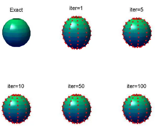
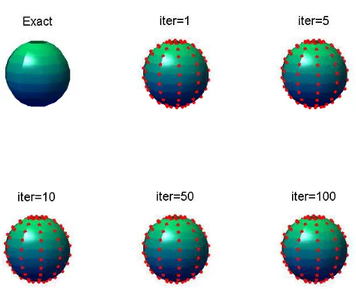
In Figures 1-3 we present the results obtained with no noise, no regularization withM =N = 6,Mf=Ne = 8,

M =N = 8,Mf=Ne = 10, M =N = 10,Mf=Ne = 12, respectively, for various numbers of iterations (iter),

as well as the correct sphere (24) to be reconstructed. From these figures it can be seen that, for exact data,

accuracy of the method is the maximum radii deviation

Er= max

n=1,N ,m=1,M|rn,m−rint|.

In Figure 4 we present the variation of Er for M = N = 6,Mf = Ne = 8, M = N = 8,Mf = Ne = 10,

M =N = 10,Mf=Ne = 12, respectively, for various numbers of iterations.

5.2

Example 2 (Cavity)

We consider again the domain Ω = Ω2\Ω1 where Ω2 andΩ1 are spheres defined by (23) and (24), respectively.

The exact solution has the form (25) but now, in order to havet1=t2=t3= 0, on the inner boundary we need

to choose the constantsAand B differently. In particular, we chooseA= 1 andB = 0.0625(1 +ν)/(1−2ν)so

that the internal sphere has radius rint= 0.5.

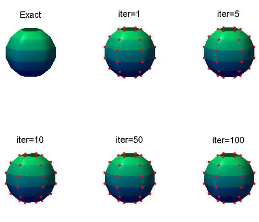
In Figures 5-7 we present the results obtained with no noise, no regularization withM =N = 6,Mf=Ne = 8,

M =N = 8,Mf=Ne = 10,M =N = 10,Mf=Ne = 12, respectively, for various numbers of iterations, as well as

the correct sphere (24) to be reconstructed. From this figure it can be seen that, for exact data, very accurate

numerical results are obtained in a relatively small number of iterations. In Figure 8 we present the variation of

Er forM =N= 6,Mf=Ne = 8, M =N= 8,Mf=Ne = 10,M =N = 10,Mf=Ne = 12, respectively, for various

numbers of iterations.

5.3

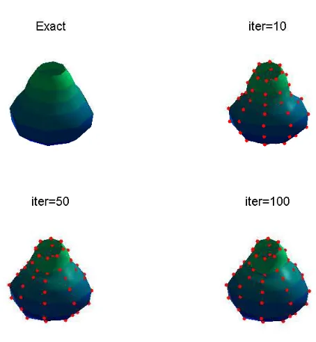
Example 3

We next consider the case R = 1, α = 1 and the rigid inclusion Ω1 has an acorn shape [23, 36] described

parametrically by

r(ϑ, ϕ) = 0.2(0.6 +√4.25 + 2 cos 3ϑ), ϑ∈(0, π), ϕ∈[0,2π), (26)

andΩ2 is the unit sphere. The Dirichlet data on∂Ω2 is taken as

uℓ(x1, x2, x3) = [

1− 2

(x2 1+x

2 2+x

2 3)

3/2 ]

xℓ, ℓ= 1,2,3, (x1, x2, x3)∈∂Ω2. (27)

Since in this case no analytical solution is available, the Neumann data (1d) is numerically simulated by solving

the direct Dirichlet well-posed problem given by equations (1a), (1b), and (1c) withα= 1, when ∂Ω1 is given

by (26), using the MFS with M =N = 20,Mf=Ne = 16. In order to avoid committing an inverse crime, the

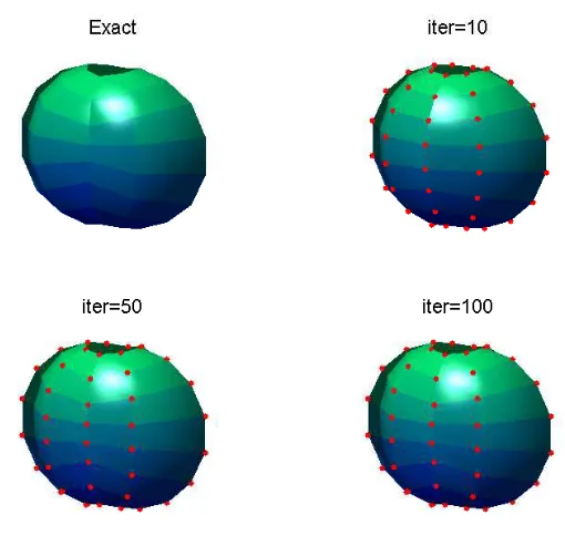
In Figures 9 and 10 we present the results obtained with X =Y = Z = 0.1, no noise and p= 5% noise,

respectively, no regularization with M =N = 8,Mf=Ne = 10, for various numbers of iterations, as well as the

correct shape (26) to be reconstructed. From Figure 9 it can be seen that for exact data, accurate retrievals of

the acorn shape (26) are obtained as the number of iterations increase, but this conclusion is not maintained for

noisy data, see Figure 10. This is because, in the absence of regularization, the obtained numerical solution will

amplify the small noise with which the input data is contaminated, thus becoming unstable. In order to deal

with this instability, regularization should be included.

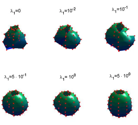
In Figures 11 and 12 we present the results obtained with noisep= 5%after 100 iterations, and regularization

withλ1 (withλ2= 0) andλ2(withλ1= 0), respectively. From Figure 11 it can be seen that regularization with

λ1is not very effective and better results are obtained for regularization withλ2, in particular whenλ2 is about

10−1_{, see Figure 12.}

Similar results have been obtained for reconstructing an acorn shape cavity, i.e. α= 0, and are therefore not

presented.

5.4

Example 4

We finally consider the case R = 1, α = 1 and the rigid inclusion Ω1 is a pinched ball [23, 36] described

parametrically by

r(ϑ, ϕ) = 0.4√1.44 + 0.5(cos 2ϑ−1) cos 2ϕ, ϑ∈(0, π), ϕ∈[0,2π), (28)

andΩ2 is the unit sphere. The Dirichlet data on∂Ω2 is taken as in (27).

Since in this case no analytical solution is available, the Neumann data (1d) is numerically simulated by

solving the direct Dirichlet well-posed problem given by equations (1a), (1b), and (1c) withα= 1, when∂Ω1is

given by (28), using the MFS withM =N =Mf=Ne = 20. In order to avoid committing an inverse crime, the

inverse solver is applied usingM =N = 8,Mf=Ne = 10.

In Figures 13 and 14 we present the results obtained with X = Y = Z = 0, no noise and p = 5% noise,

respectively, no regularization with M =N = 8,Mf=Ne = 10, for various numbers of iterations, as well as the

correct shape (28) to be reconstructed. The same conclusions as those discussed for Example 3 from Figures 9

and 10 above can be drawn from Figures 13 and 14 for Example 4.

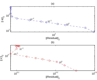
withλ1 (withλ2= 0) andλ2 (withλ1= 0), respectively. Finally, in Figure 17 we present the corresponding

L-curves withλ1andλ2regularizations for noisep= 5%after 100 iterations. The L-curve corner for regularization

inλ1is not consistent with the best results which appear just aboveλ1= 10−1 in Figure 15 whereas the L-curve

corner for regularization inλ2 is consistent with the the best results which appear around λ2 = 10−1 in Figure

16.

6

Conclusions

The main features of this work can be summarized as follows:

• This is the first time a three-dimensional inverse geometric problem in elasticity has been considered using

the MFS.

• We get the full benefits of the MFS since we are dealing with a nonlinear problem in three dimensions and in

complex geometries. Here, the meshlessness and the boundary nature of the method and their concomitant

ease of implementation become important.

• The numerical results indicate that the numerical method is accurate (for no noise) and stable with respect

to noise added in the input data.

• Accurate results are obtained for relatively few degrees of freedom.

• The dynamic approach of the MFS has been used. It is well-suited for such nonlinear problems since, in

addition to the parameters determining the shape of the sought void, we simultaneously determine the

location of the unknown pseudo-boundaries as well as the coordinates of the centre of the object.

• The MFS implementations to three-dimensional isotropic linear thermo-elasticity, as well as to two- and

three-dimensional anisotropic linear elasticity, of the corresponding inverse void problems are deferred to a

future work.

Acknowledgements. _{Liviu Marin acknowledges the financial support received from the Romanian National}

References

[1] G. Alessandrini, A. Bilotta, G. Formica, A. Morassi, E. Rosset, and E. Turco,Numerical size estimates of

inclusions in elastic bodies, Inverse Problems21_{(2005), 133–151.}

[2] G. Alessandrini, A. Morassi, and E. Rosset,Detecting an inclusion in an elastic body by boundary

measure-ment, SIAM J. Math. Anal.33 _{(2002), 1247–1268.}

[3] C. J. S. Alves and N. F. M. Martins,The direct method of fundamental solutions and the inverse

Kirsch-Kress method for the reconstruction of elastic inclusions or cavities, J. Integral Equations Appl. 21_(2009),

153–178.

[4] D. D. Ang, D. D. Trong, and M. Yamamoto,Identification of cavities inside two-dimensional heterogeneous

isotropic elastic bodies, J. Elasticity56_{(1999), 199–212.}

[5] P. K. Banerjee and R. Butterfield,Boundary Element Methods in Engineering Science, McGraw-Hill Book

Co. (UK), Ltd., London-New York, 1981.

[6] M. R. Barone and R. J. Yang, A boundary element approach for recovery of shape sensitivities in

three-dimensional elastic solids, Comput. Methods Appl. Mech. Engrg.74 _{(1989), 69–82.}

[7] H. Ben Ameur, M. Burger, and B. Hackl,Level set methods for geometric inverse problems in linear elasticity,

Inverse Problems20 _{(2004) 673–696.}

[8] H. Ben Ameur, M. Burger, and B. Hackl,Cavity identification in linear elasticity and thermoelasticity, Math.

Methods Appl. Sci.3_{(2007), 625–647.}

[9] L. M. Bezerra and S. A. Saigal,Boundary element formulation for the inverse elastostatics problem (IESP)

of flaw detection, Internat. J. Numer. Methods Engrg.36_{(1993), 2189–2202.}

[10] M. Bonnet and A. Constantinescu, Inverse problems in elasticity, Inverse Problems21_{(2005), R1–R50.}

[11] M. Bonnet and B. J. Guzina,Elastic-wave identification of penetrable obstacles using shape-material

sensi-tivity framework, J. Comput. Phys.228_{(2009), 294–311.}

[12] D. Borman, D. B. Ingham, B. T. Johansson, and D. Lesnic, The method of fundamental solutions for

[13] T. F. Coleman and Y. Li,On the convergence of interior-reflective Newton methods for nonlinear

minimiza-tion subject to bounds, Math. Programming67_{(1994), 189–224.}

[14] T. F. Coleman and Y. Li,An interior trust region approach for nonlinear minimization subject to bounds,

SIAM J. Optim.6_{(1996), 418–445.}

[15] P. Gorzelańczyk and J. A. Kołodziej,Some remarks concerning the shape of the source contour with

appli-cation of the method of fundamental solutions to elastic torsion of prismatic rods, Eng. Anal. Bound. Elem.

37_{(2008), 64–75.}

[16] J. Hadamard, Lectures on Cauchy Problem in Linear Partial Differential Equations. Yale University Press,

New Haven, 1923.

[17] F. Hartmann, Elastostatics, Progress in Boundary Element Methods. Vol. 1 (C. A. Brebbia, ed.), Pentech

Press, London, 1981, pp. 84–167.

[18] S.-C. Hsieh and T. Mura,Nondestructive cavity identification in structures, Int. J. Solids Struct.30_(1993),

1579–1587.

[19] M. Ikehata and H. Itou,Extracting the support function of a cavity in an isotropic elastic body from a single

set of boundary data, Inverse Problems25_{(2009), 105005.}

[20] A. Karageorghis, D. Lesnic, and L. Marin,A survey of applications of the MFS to inverse problems, Inverse

Probl. Sci. Eng.19_{(2011), 309–336.}

[21] A. Karageorghis, D. Lesnic, and L. Marin, The method of fundamental solutions for the detection of rigid

inclusions and cavities in plane linear elastic bodies, Comput. & Structures 106-107_{(2012), 176–188.}

[22] A. Karageorghis, D. Lesnic, and L. Marin,A moving pseudo-boundary method of fundamental solutions for

void detection, Numer. Methods Partial Differential Equations29_{(2013), 935–960.}

[23] A. Karageorghis, D. Lesnic, and L. Marin, A moving pseudo-boundary MFS for three-dimensional void

detection, Adv. Appl. Math. Mech.5_{(2013), 510–527.}

[24] A. J. Kassab, F. A. Moslehy, and A. B. Daryapurkar, Nondestructive detection of cavities by an inverse

[25] A. Kirsch and R. Kress, On an integral equation of the first kind in inverse acoustic scattering, Int. Ser.

Numer. Math.77_{(1986), 93–102.}

[26] V. D. Kupradze and M. A. Aleksidze, The method of functional equations for the approximate solution of

certain boundary value problems, Comput. Math. Math. Phys.4_{(1964), 82–126.}

[27] D. Lesnic, J. R. Berger, and P. A. Martin, A boundary element regularization method for the boundary

determination in potential corrosion damage, Inverse Probl. Eng.10_{(2002), 163–182.}

[28] L. Marin, Regularized method of fundamental solutions for boundary identification in two-dimensional

isotropic linear elasticity, Int. J. Solids Struct. 47_{(2010), 3326–3340.}

[29] L. Marin, and D. Lesnic, BEM first-order regularisation method in linear elasticity for boundary

identifica-tion, Comput. Methods Appl. Mech. Engrg. 192_{(2003), 2059–2071.}

[30] S. C. Mellings and M. H. Aliabadi, Flaw identification using the boundary element method, Internat. J.

Numer. Methods Engrg.38_{(1995), 399–419.}

[31] R. Mathon and R. L. Johnston,The approximate solution of elliptic boundary value problems by fundamental

solutions, SIAM J. Numer. Anal.14 _{(1977), 638–650.}

[32] The MathWorks, Inc., 3 Apple Hill Dr., Natick, MA,Matlab.

[33] A. Morassi and E. Rosset,Detecting rigid inclusions, or cavities, in an elastic body, J. Elasticity 73_(2003),

101–126.

[34] A. Morassi and E. Rosset,Uniqueness and stability in determining a rigid inclusion in an elastic body, Mem.

Amer. Math. Soc.200_{(2009), 58pp.}

[35] A. Poullikkas, A. Karageorghis, and G. Georgiou,The method of fundamental solutions for three-dimensional

elastostatics problems, Comput. & Structures80 _{(2002), 365–370.}

[36] P. Serranho,A hybrid method for inverse scattering for sound-soft obstacles in R3_{, Inverse Probl. Imaging}

1_{(2007), 691–712.}

[37] T. W. Ulrich, F. A. Moslehy, and A. J. Kassab,A BEM based pattern search solution for a class of inverse

Figure 2: Example 1: Results for M =N = 8,Mf=Ne = 10, no noise and no regularization.

0 20 40 60 80 100 10−4

10−3 10−2 10−1 100

iter

E

r

M=N=6 M=N=8 M=N=10

Figure 4: Example 1: Variation of errorEr with the number of iterations.

Figure 6: Example 2: Results for M =N = 8,Mf=Ne = 10, no noise and no regularization.

0 20 40 60 80 100 10−3

10−2 10−1 100

iter

E

r

M=N=6 M=N=8 M=N=10

Figure 8: Example 2: Variation of errorEr with the number of iterations.

Figure 10: Example 3: Results forM =N= 8,Mf=Ne = 10, noisep= 5%and no regularization.

Figure 12: Example 3: Results forM =N = 8,Mf=Ne = 10, noisep= 5%and regularization withλ2.

Figure 14: Example 4: Results forM =N= 8,Mf=Ne = 10, noisep= 5%and no regularization.

Figure 16: Example 4: Results forM =N= 8,Mf=Ne = 10, noisep= 5%and regularization withλ2.

101 101

102

10−2

10−1

100

||Residual||₂

||

c

|| 2

(a)

100.1 100.2 100.3

100 10 −1

10−2

100

||Residual|| 2

||

r

′ || 2

(b)