Point Spread Function and Modulation Transfer Function Engineering

Rochester Institute of Technology

RIT Scholar Works

Theses

8-23-2019

Point Spread Function and Modulation Transfer

Function Engineering

Jacob Wirth

Follow this and additional works at:

https://scholarworks.rit.edu/theses

This Dissertation is brought to you for free and open access by RIT Scholar Works. It has been accepted for inclusion in Theses by an authorized administrator of RIT Scholar Works. For more information, please contactritscholarworks@rit.edu.

Recommended Citation

by

Jacob Wirth

B.A. State University of New York at Geneseo, 2014

A dissertation submitted in partial fulfillment of the

requirements for the degree of Doctor of Philosophy

in the Chester F. Carlson Center for Imaging Science

College of Science

Rochester Institute of Technology

August 23, 2019

Signature of the Author

Accepted by

CHESTER F. CARLSON CENTER FOR IMAGING SCIENCE

COLLEGE OF SCIENCE

ROCHESTER INSTITUTE OF TECHNOLOGY

ROCHESTER, NEW YORK

CERTIFICATE OF APPROVAL

Ph.D. DEGREE DISSERTATION

The Ph.D. Degree Dissertation of Jacob Wirth has been examined and approved by the dissertation committee as satisfactory for the

dissertation required for the Ph.D. degree in Imaging Science

Dr. Grover Swartzlander, Dissertation Advisor

Dr. Stefan Preble, External Chair

Dr. Zoran Ninkov

Dr. Abbie Watnik

Date

COLLEGE OF SCIENCE

CHESTER F. CARLSON CENTER FOR IMAGING SCIENCE

Title of Dissertation:

Point Spread Function and Modulation Transfer Function Engineering

I, Jacob Wirth, hereby grant permission to Wallace Memorial Library of R.I.T. to

reproduce my thesis in whole or in part. Any reproduction will not be for commercial

use or profit.

Signature

Date

Point Spread Function and Modulation Transfer Function

Engineering

by

Jacob Wirth

Submitted to the

Chester F. Carlson Center for Imaging Science in partial fulfillment of the requirements

for the Doctor of Philosophy Degree at the Rochester Institute of Technology

Abstract

A novel computational imaging approach to sensor protection based on point spread

func-tion (PSF) engineering is designed to suppress harmful laser irradiance without significant

loss of image fidelity of a background scene. PSF engineering is accomplished by modifying

a traditional imaging system with a lossless linear phase mask at the pupil which diffracts

laser light over a large area of the imaging sensor. The approach provides the additional

advantage of an instantaneous response time across a broad region of the electromagnetic

spectrum. As the mask does not discriminate between the laser and desired scene, a post-processing image reconstruction step is required, which may be accomplished in real time,

that both removes the laser spot and improves the image fidelity.

This thesis includes significant experimental and numerical advancements in the

de-termination and demonstration of optimized phase masks. Analytic studies of PSF

engi-neering systems and their fundamental limits were conducted. An experimental test-bed

was designed using a spatial light modulator to create digitally-controlled phase masks to

image a target in the presence of a laser source. Experimental results using already known

phase masks: axicon, vortex and cubic are reported. New methods for designing phase

masks are also reported including (1) a numeric differential evolution algorithm, (2) a PSF reverse engineering method, and (3) a hardware based simulated annealing experiment.

Broadband performance of optimized phase masks were also evaluated in simulation.

Op-timized phase masks were shown to provide three orders of magnitude laser suppression

Acknowledgements

I would like to first acknowledge the Office of Naval Research for supporting this research. This work was also supported by the Chester F. Carlson Center for Imaging Science at the

Rochester Institute of Technology. I would also like to acknowledge American Society for

Engineering Education who provided the support allowing me to conduct this work at the

Naval Research Laboratory through the Naval Research Enterprise Internship Program.

I am eternally grateful to all the individuals who gave me their time throughout this

process. First I would like to thank my advisers: Grover Swartzlander and Abbie Watnik.

You both challenged and supported me over the past 5 years. I am truly a better researcher

and scientist because of you and I hope to make you both proud with my future accom-plishments. I also thank the remainder of my dissertation committee, Zoran Ninkov and

Stefan Preble, for their counsel and encouragement. I would also like to thank those who

helped me during my temporary internships at the Naval Research Laboratory including

Colin Olson and Tim Doster. I would also like to thank the collaborators of this work Erin

Fleet and Kyle Novak for many fruitful conversations.

Thank you to my friends and labmates who provided many words of encouragement and

laughter. Thank you to my Mom and Dad who supported me in both my accomplishments

and failures and who gave me every opportunity to succeed. Finally I am thankful to

Maxine who helped make me the best version of myself.

1.1 Basic PSF engineered imaging system schematic. . . 5

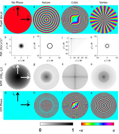
1.2 Pupil, PSF, and OTF for the axicon, cubic, and vortex phase functions . . 12

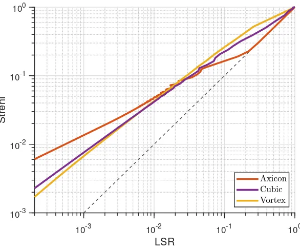
1.3 Strehl vs LSR for the axicon, cubic, and vortex phase functions. . . 13

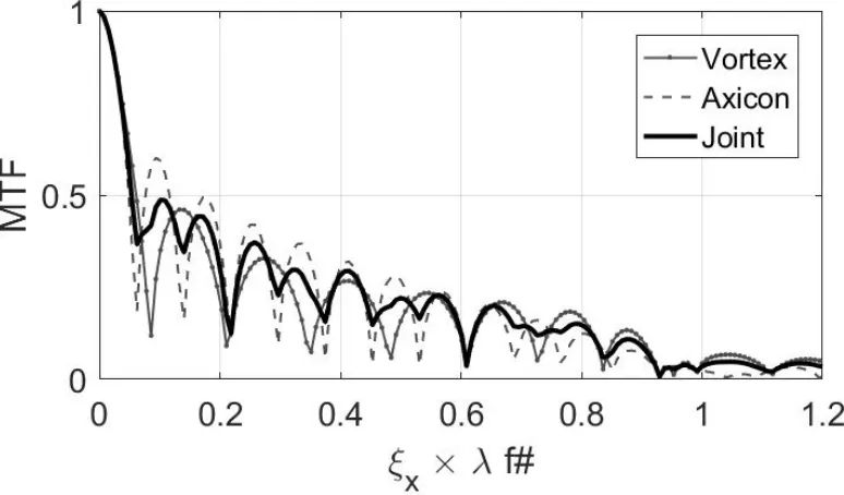
2.1 MTF line profiles showing removal of null from a joint deconvolution . . . . 24

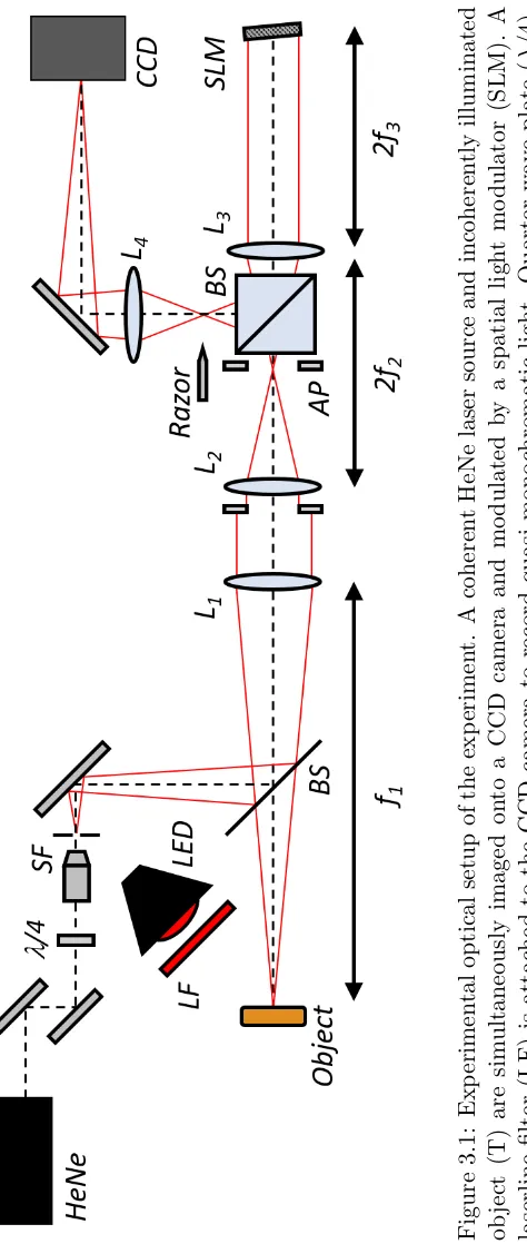
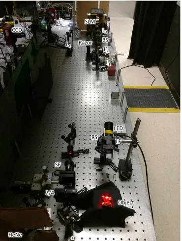
3.1 The experimental setup . . . 28

3.2 Photo of the experimental setup. . . 30

3.3 Diagram of a liquid crystal . . . 31

3.4 Cross section of the liquid crystal on silicon (LCOS) SLM. . . 33

3.5 Simulation of ghost image from SLM . . . 34

3.6 SLM deflection technique for removing unwanted specular reflection . . . . 35

3.7 Ray Trace of multiple diffractive orders of the SLM . . . 36

3.8 High speed images of SLM flicker . . . 37

3.9 PSF before and after wavefront correction . . . 39

3.10 Example phase correction for SLM . . . 39

3.11 Experimentally recorded PSFs and respective MTFs for axicon, vortex, and cubic phase functions . . . 41

LIST OF FIGURES viii

3.12 Experimental images of target using axicon, vortex, and cubic phase functions 42

3.13 Line profiles of Fig. 3.12. . . 44

3.14 Edge response and noise gain measurements for axicon, vortex, and cubic images. . . 45

4.1 Strehl/LSRmap for two example basis phase functions . . . 48

4.2 Pupil Phase, PSF, and OTF for mask optimized via differential evolution . 54 4.3 Numerically calculated image quality metrics for masks optimized via dif-ferential evolution . . . 56

4.4 Experimental images using masks optimized via differential evolution . . . . 58

4.5 Experimentally derived image quality metrics for masks optimized via dif-ferential evolution . . . 59

4.6 The Strehl ratio for optimized azimuthal harmonic phase functions . . . 61

4.7 Pupil phase, PSF, MTF, and phase transfer functions for the azimuthal harmonic phase functions . . . 62

4.8 Pupil phase, PSF, and MTF before and after simulated annealing algorithm 64 4.9 Iterations of the simulated annealing algorithm . . . 65

4.10 Strehl, LSR, and Strehl/LSR as a function of iteration as calculated from the experimental images. . . 66

4.11 Half ring PSF and even and odd components . . . 68

4.12 Half ring MTF and real and imaginary components . . . 69

4.13 OTF zero crossings for half ring PSF . . . 70

4.14 Numeric and analytic OTF for half ring PSF . . . 73

4.15 OTF line profiles for half ring PSF . . . 74

4.17 Optimized five half ring PSF . . . 77

4.18 Half axicon pupil phase and PSF . . . 78

4.19 Holographic approximation of half ring pupil phase . . . 79

4.20 Strehl vs LSR plot for half ring PSF functions . . . 81

4.21 Pupil phase for five half ring PSF through holographic estimate and iterative phase retrieval . . . 82

4.22 Graphical representation of the Gerchberg-Saxton phase retrieval algorithm 83 4.23 Comparison of estimated five half ring PSFs . . . 84

4.24 Strehl vs LSR plot summarizing the performance of each of the optimized PSFs. . . 86

4.25 pupil phase, PSF, and OTF for optimized phase masks . . . 89

4.26 Targets to be imaged in experiment . . . 90

4.27 Experimental images of clay figurine . . . 91

4.28 Experimental images of resolution bar target . . . 92

4.29 Line profiles of Fig. 4.28 . . . 94

4.30 Noise gain and edge response for experimental images with optimized phase functions . . . 95

4.31 Experimental images with optimized phase functions and laser present . . . 96

4.32 Experimental images with laser present processed with laser removal algorithm 98 5.1 The integrated broadband PSF and MTF for the azimuthal harmonic phase function. . . 107

LIST OF FIGURES x

5.4 Process for simulating panchromatic images using a hyperspectral data set. 111

2.1 Odd and Even symmetries of OTF and PSF based on symmetry of pupil phase . . . 22

3.1 Specifications for spatial light modulators used in this work. . . 33

3.2 Experimentally measured laser suppression of axicon, vortex, and cubic

phase functions . . . 40

4.1 Parameters and results of differential evolution optimizations . . . 53

4.2 Values ofγ fit via Eq. 4.29 for phase masks and PSFs studied in this thesis 87

List of Acronyms

BS Beam Splitter.

CCD Charge-Coupled Device.

DEA Differential Evolution Algorithm.

FT Fourier Transform.

GIQE General Image Quality Equation.

LC Liquid Crystal.

LCOS Liquid Crystal on Silicon.

LED Light Emitting Diode.

LF Laserline Filter.

LSR Light Suppression Ratio.

MTF Modulation Transfer Function.

NG Noise Gain.

NIIRS National Imagery Interpretability Rating Scale.

NM Nelder Mead.

OTF Optical Transfer Function.

PSF Point Spread Function.

PTF Phase Transfer Function.

RER Relative Edge Response.

SF Spatial Filter.

SLM Spatial Light Modulator.

Contents

1 Background 1

1.1 Motivation . . . 1

1.2 Fourier Optics . . . 4

1.3 Deconvolution . . . 7

1.4 Image Quality Metrics . . . 8

1.5 Basic Phase Functions . . . 10

1.6 Outline of Thesis . . . 14

2 Point Spread Function Engineering Theory 15 2.1 Strehl Ratio Limits . . . 16

2.2 Odd and Even Pupil function Taxonomy . . . 18

2.2.1 Even and Odd Functions and their Fourier transforms . . . 19

2.2.2 Odd/Even Pupil Functions . . . 20

2.3 Joint Deconvolution . . . 22

2.4 Summary . . . 24

3 Experimental System and Implementation 26 3.1 Experimental Setup . . . 27

3.2 Spatial Light Modulator . . . 31

3.2.1 SLM Background . . . 31

3.2.2 Limitations of the SLM . . . 33

3.3 Experimental Validation . . . 39

3.4 Summary . . . 44

4 Pupil Phase Optimization 47 4.1 Global Optimization: Differential Evolution . . . 50

4.1.1 Differential Evolution Validation . . . 57

4.1.2 Azimuthal Harmonic Phase Functions . . . 60

4.2 Hardware Based Optimization: Simulated Annealing . . . 61

4.3 PSF Reverse Engineering . . . 67

4.3.1 Multi Ring PSF . . . 73

4.3.2 Half Ring Pupil Phase . . . 75

4.3.3 Multi Half Ring Pupil Phase . . . 80

4.3.4 Half Ring PSF Summary . . . 84

4.4 Optimized PSF Summary . . . 85

4.5 Experimental Validation and Comparison . . . 88

4.5.1 Images Saturated by Laser Source . . . 96

4.6 Summary . . . 97

5 Broadband Considerations 101 5.1 Broadband Imaging Theory . . . 101

5.2 The Broadband PSF . . . 102

5.3 Broadband Imaging Simulation . . . 110

CONTENTS xvi

6 Conclusion and Future Directions 115

6.1 Conclusion . . . 115 6.2 Future Directions . . . 117

A Circularly Symmetric Functions 118

Background

1.1

Motivation

Since the invention of the laser, there has been concern over its potential to damage and

disrupt sensors. For decades, research has been conducted on more compact systems and increasing laser powers including the infamous “Star Wars” strategic defense initiative [1,2].

While in the past the dream of laser weapons have been out of reach, systems have now had

successful field tests are now being developed for deployment [3]. The HELIOS program is

set to be deployed as soon as 2020 with a power of up to 150 kW - capable of dazzling or

damaging imaging sensors more than 3 km away [4, 5]. As laser powers continue to grow,

a proliferation of laser weapons should be expected.

As these laser systems become increasingly common, effective countermeasures are

necessary for protecting sensors from potential dazzle and damage. Traditional methods for

attenuating high intensity lasers in the laboratory such as neutral density filters, bandpass filters, polarizers, or mechanical shutters will equally affect the background scene, require

prior knowledge of the laser’s wavelength or polarization state, or required detection of

CHAPTER 1. BACKGROUND 2

the laser. Coronagraphs, useful for imagining dim exoplanets near a bright overwhelming

star, require accurate pointing [6–8]. Mechanisms for deflecting potentially damaging or dazzling laser light using micro mirror devices have been developed, but are bulky and

require prior detection of the laser [9, 10]. Optical limiters provide a promising method

of laser suppression [11–27]. Such devices leverage nonlinear transmission of materials to

limit laser throughput. However, optical limiters have limited spectral bandpass, a nonzero

response time, and can degrade the image. New methods are necessary to overcome these

issues.

This thesis describes a novel computational imaging approach to sensor protection based

on point spread function (PSF) engineering. A mask is introduced to the pupil plane of a

traditional imaging system which redistributes the incident laser beam over a larger area of the sensor reducing the peak irradiance and effectively protecting the sensor from damage.

As the mask does not discriminate between harmful laser radiation and the desired scene,

a post-processing step is required to remove saturated pixels and restore the image.

PSF engineering has been used for improving and adding functionality to imaging

systems. Coded apertures using binary patterns have been studied for reducing the affects

of aberrations on imaging systems and improving optical resolution [28–31]. More recently,

the use of phase-only masks have been used to modify the PSF without affecting the

throughput of the imaging system. Phase masks have been demonstrated to extend the

depth of field of an imaging system [32–35] and to encode 3D information using rotating PSFs [36–41].

Linear phase elements are capable of providing instantaneous laser suppression over

a large bandwidth of the electro-magnetic spectrum. High damage threshold phase

subwavelength patterned surfaces include polarization diffraction gratings and

metasur-faces [51–57]. Each of these have been implemented for designing mask with arbitrary phase patterns.

A desirable point spread function has a low peak amplitude and retains a high amount

of information from the scene. These qualities are often considered a trade-off from one

another, but this work has found that PSFs with the same peak amplitude can have vastly

different fidelity of restored images. This thesis includes significant experimental and

nu-merical advancements in the determination and demonstration of optimized phase masks.

Analytic studies of PSF engineering systems in terms of the integrated Strehl ratio with

fundamental limits are found. An experimental test-bed was designed to validate imaging

performance using a spatial light modulator to create digitally-controlled phase masks to image a target in the presence of a laser source. Experimental results using already known

phase masks: axicon, vortex and cubic are reported. Numeric and analytic approaches

were taken to optimize the phase mask and PSF including (1) a numeric differential

evolu-tion algorithm, (2) a PSF reverse engineering method, and (3) a hardware based simulated

annealing experiment. The PSF reverse engineering method was especially successful

pro-viding a new family of PSFs: half-ring PSFs which resulted in the highest imaging fidelity

relative to level of laser suppression. Broadband performance of optimized phase masks

were also evaluated in simulation. Optimized phase masks were experimentally shown to

CHAPTER 1. BACKGROUND 4

1.2

Fourier Optics

We consider an imaging system as depicted in Fig. 1.1 comprising an incoherently

illumi-nated object or scene, a lens of focal lengthf and aperture function A(x, y), and a sensor

in the image plane. A phase mask having transmittance function t(x, y) is placed at the entrance face of the lens. Superimposed upon the scene is a laser source which diffracts

over free space to form a planar wavefront at the entrance face of the lens. Both the scene

distancezand the characteristic laser diffraction lengthzRare assumed to be much greater

than the focal lengthf. For a non-uniform phase mask (e.g., t(x, y)6= 1) the point spread

function of the imaging system becomes blurred or distorted, thereby reducing the risk of

damage to the focal plane sensor. For a well-designed phase mask, the blurred image of

scene can be reconstructed using deconvolution post-processing techniques. The objective

of this research is to determine a means of spreading the laser power across a large area,

thereby reducing the risk of damage, while simultaneously being able to restore a high fidelity.

The PSF of the system, h(x0, y0), is the Fourier transform of the pupil of the system

h(x0, y0) =F T[A(x, y)t(x, y)] =

Z ∞

−∞

Z ∞

−∞

A(x, y)t(x, y)×exp[−i2π λf(x

0

x+y0y)]dxdy (1.1)

where λ is the wavelength of light. The incoherent PSF is |h(x0, y0)|2_{. Below we assume}

the maximum value ofA(x, y) and |t(x, y)|is unity.

Figure 1.1: Basic PSF engineered imaging system schematic. A distant scene comprised of an incoherent background intensity,Ib(x0, y0), and coherent laser field,Ul(x0, y0) is imaged

with a lens of aperture radiusRhaving an adjacent pupil plane maskt(x, y). The resulting detected image is blurred and is restored in post-processing.

Ul(x0, y0), and the coherent PSF

U_l0(x0, y0) =

Z Z

Ul(u, v)h(u−x0, v−y0)dudv =Ul(x0, y0)⊗h(x0, y0) (1.2)

The same is true for the geometric image of the background sceneIb(x0, y0), and incoherent PSF.

I_b0(x0, y0) =Ib(x0, y0)⊗ |h(x0, y0)|2 (1.3)

whereIb(x0, y0) is the geometric profile of sceneIb(x0, y0). The measured intensity may be

expressed as the sum of the coherent and incoherent components as

Imeas(x0, y0) =|Ul0(x0, y0)|2+Ib0(x0, y0). (1.4)

CHAPTER 1. BACKGROUND 6

greater than the Rayleigh range,zR=πw20/λ, wherew0 is the waist of the laser. The laser

field at the pupil of the system may then be represented as a tilted plane wave with uniform illumination over the aperture which may be represented byU0exp[ik(αx+βy)] whereU0

is a scalar amplitude, andαandβ are tip and tilt angles. This results in a geometric image

of a shifted point represented by a dirac delta,Ul(x0, y0) =δ(x0−αf, y0−βf). The Fourier transform of Eq. 1.4 represents the power spectrum,Smeas(ξx, ξy), of the detected image:

Smeas(ξx, ξy) =F T[Imeas(x0, y0)] =

{F T[δ(x0−αf, y0−βf)] +Sb(ξx, ξy)} ×H(ξx, ξy) (1.5)

where ξx = x/λf and ξy = y/λf are spatial frequency coordinates and Sb(ξx, ξy) is the

power spectrum of the geometric background image, and H(ξx, ξy) is the optical transfer

function (OTF) defined as

H(ξx, ξy) =F T[|h(x0, y0)|2] =

Z ∞

−∞

Z ∞

−∞

|h(x0, y0)|2_{exp[−i2π(x}0_ξ

x+y0ξy)]dx0dy0. (1.6)

The magnitude |H(ξx, ξy)| is the modulation transfer function (MTF) which provides a

measure of how the spatial frequencies of the geometric image are reduced in the final detected image.

The relationship between the pupil function, PSF, and OTF is nonlinear and complex

resulting in the difficult problem of optimizing each function to provide the ideal system

[58]. Two functions may provide the same laser suppression, but result in different image

qualities. The integration of two MTF’s may be the same, but their different distributions

1.3

Deconvolution

In processing the image, the goal is to restore Ib(x0, y0) through deconvolution. Using Eq. 1.5, this process can be done by dividing the spectrum of the final recorded image,

Smeas(ξx, ξy), by the OTF of the system, H(ξx, ξy). Subtracting the laser contribution from the result will leave only the the incoherent scene. This process is known as inverse

filtering.

In reality, the true recorded spectrum will contain some amount of noise from

vari-ous sources such as Poisson noise, air turbulence, and detector noise. Adding the noise

contribution, the resulting spectrum may be represented as

Smeas(ξx, ξy) = [Sl(ξx, ξy) +Sb(ξx, ξy)]×H(ξx, ξy) +N(ξx, ξy)

=Stot(ξx, ξy)×H(ξx, ξy) +N(ξx, ξy) (1.7)

where N(ξx, ξy) represents the total noise in the image and Stot(ξx, ξy) is the sum of the

laser and scene spectra. Inverse filtering, dividing Eq. 1.7 by the OTF, results in:

Smeas(ξx, ξy) H(ξx, ξy)

=Stot(ξx, ξy) +

N(ξx, ξy) H(ξx, ξy)

. (1.8)

The contributionN(ξx, ξy)/H(ξx, ξy) leaves a high amount of noise gain when|H(ξx, ξy)|<<

1 which would greatly degrade the restored image.

A method for restoring the image while considering the added noise must be used. Let

Se(ξx, ξy) be the spectrum calculated from the experimentally recorded image. Consider

the total error betweenSe(ξx, ξy) and Eq. 1.7.

E=

Z Z

CHAPTER 1. BACKGROUND 8

Minimizing the error and solving forStot(ξx, ξy) results in

Sb(ξx, ξy) =Se(ξx, ξy)

H∗(ξx, ξy)

|H(ξx, ξy)|2+ 1/SN R(ξx, ξy)

=Se(ξx, ξy)W(ξx, ξy) (1.10)

where W(ξx, ξy) is the Wiener filter and SN R(ξx, ξy) is the signal to noise ratio as a

function of spatial frequency. This process, called Wiener deconvolution, seeks to dampen the effect of noise on the final restored image [59]. Note that when the noise is zero, the

Wiener filter becomes the inverse filter. In practice, the value of SNR may be an adjustable

parameter rather than the experimentally determined function.

1.4

Image Quality Metrics

The system performance is categorized by 1) how much the intensity on the sensor is

reduced and 2) the quality of the final image. We define a new quantitative metric, the

light suppression ratio (LSR), which quantifies how much the sensor is protected. It is

defined as the normalized peak value of the incoherent PSF or

LSR= max[|h(x

0_{, y}0_)|2_]

max[|h0(x0, y0)|2]

(1.11)

where |h0(x0, y0)|2 is the diffraction-limited PSF. Through this work, an LSR is sought

which protects a sensor for several orders of magnitude.

To quantify image quality, several metrics were considered. The National Imagery

Interpretability Rating Scale (NIIRS) is the method the remote sensing and intelligence

community uses for ranking satellite imagery [60]. Traditionally, a value from 0 to 9 is

equation (GIQE) was created to estimate the NIIRS value by combining several

quanitifi-able metrics of an imaging system and is defined as

N IIRS =c0+c1log10(GSD) +c2log10(RER)−c3G/SN R+c4H (1.12)

where RER is the relative edge response, GSD is the ground sample distance, H is the edge overshoot, andGis the noise gain [61]. The values of cwere found by fitting Eq. 1.12

to set of images in which NIIRS values had previously been assigned.

In the case of the PSF engineered system described in this work, the GIQE would be an

extreme extrapolation of this fit as none of the images in the data set utilize PSF engineered

reconstructions. In fact, the GIQE has been found inaccurate for highly aberrated images

and those restored through deconvolution [62]. In addition, the metrics used as input values

are empirical and require prior knowledge of the system includingGSD and SN R. Direct

measurements are also required forRERandHfor specific edges while the engineered PSF

may have a different performance on each edge. In Ref. [62], the RER and G terms are identified as the important parameters of the GIQE for restored imagery. For experimental

images, these terms will be used to quantify the image quality. For predicting the fidelity

of restored images in simulation, a different, more fundamental image quality metric is

sought.

The Strehl ratio is a commonly used method for quantifying image quality. Generally,

this value is calculated as the on axis peak intensity of the PSF normalized by the PSF [63].

In this work, an alternate definition of the Strehl ratio is used which is calculated from the

MTF [64]

Strehl=

R R

|H(ξx, ξy)|dξxdξy

R R

|H0(ξx, ξy)|dξxdξy

CHAPTER 1. BACKGROUND 10

where H0(ξx, ξy) is the diffraction limited OTF. It was found that different phase masks

with the same LSR may provide varying values for the integrated Strehl ratio. In addition, no empirical information of the imaging system is required.

A phase function is sought which maximizes the ratio Strehl/LSR. This problem

containing three functions which are related nonlinearly: the pupil function, OTF, and

PSF. As there is no known analytic solution, various numeric and analytic techniques are

implemented to optimize the ratio.

1.5

Basic Phase Functions

To begin studying PSF engineered imaging systems, phase-only elements with long standing

applications are observed. These elements include: axicons used for creating “diffraction

free” bessel beams [57, 65], cubics used to enhance the depth of focus for wavefront coded

systems [32, 34, 35], and vorticies which contain angular momentum and are used in optical

trapping, coronagraphs, and communication [6, 66–68]. The phase functions for these

elements are defined as

Φaxicon(x, y) =ar/R (1.14a)

Φcubic(x, y) = 2πb(x3+y3)/R3 (1.14b)

Φvortex(x, y) =mθ (1.14c)

where a, b, and m are scaling parameters which alter the phase gradient and R is the

aperture radius. By increasing the phase gradient, the light is diffracted over a larger area

on the focal plane which reduces the peak intensity. To do so comes at a potential cost to

the fidelity of a restored image.

calculated via a Fast Fourier Transform (FFT) [69]. An NxN pixel computational grid is

created with N = 4096. The pupil is defined by a circular aperture with radius ar = 512 pixels and is multiplied by the phase functionexp[iΦ(x, y)]. The phase functions in Eq. 1.14

are each easily normalized relative to the radius of the aperture (r/R). The FFT of the

pupil is taken and the magnitude squared is taken to find the incoherent PSF. The inverse

FFT is taken of incoherent PSF to calculate the OTF.

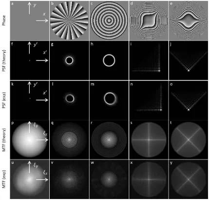
This process was implemented to calculate the PSF and OTF for several phase masks

in the pupil: no phase, an axicon with a= 40, a cubic with value b = 15, and a vortex

with value m= 20. The results are shown in Fig. 1.2. Each of the images are shown in a

normalized coordinate space where the edge of the pupil (first row) is the coherent cutoff

frequency,ξ0 = 1/2λf# whereλis the wavelength of light,f# =f /2R, andf is the focal

length. The edge of the MTF (third row) is the incoherent cutoff frequency. The second

row shows the PSF and the fourth row the phase transfer function.

The axicon and vortex phase functions produce ring-like PSFs, with the axicon having

a narrower annulus. The cubic produces a fan-like structure with an intense peak at the

vertex. Both the vortex and axicon MTF’s contain zeros as concentric rings. These zeros

represent a total loss of information from the scene to the image. The cubic has most of

the MTF concentrated on two perpendicular axes which may be good for imaging scenes

which have a lot of perpendicular edges, but the PSF has a much greater extent which may

CHAPTER 1. BACKGROUND 12

10-3 10-2 10-1 100

LSR

10-3 10-2 10-1

Strehl

Figure 1.3: A plot of Strehl vs LSR for the axicon, cubic, and vortex phase functions.

The integrated Strehl ratio is calculated from the numeric MTFs by summing the pixel

values and normalizing by the sum of the no phase MTF pixels. The LSR is calculated

from the peak intensity of the PSF normalized by the no phase case. By altering the phase

gradients (a, b, and m), continuous curves are generated for each phase function. The

results are shown in Fig. 1.3. At any given value of LSR, Fig. 1.3 shows different phase

functions can have vastly different integrated Strehl ratios. For values of LSR greater than

0.02, the vortex phase mask has the highest value of Strehl. For values of LSR less than

0.02, the axicon has the highest value of Strehl. Despite this, the nulls in the MTFs for

the vortex and axicon phase functions will result in reconstructed images with a high noise gain.

CHAPTER 1. BACKGROUND 14

points for the axicon, cubic, and vortex, phase functions were chosen for examples shown in

Fig. 1.2. Studying these three masks will provide insight beyond the value for Strehl. The phase functions at a value for LSR of 0.02 are to be compared experimentally to observe

their respective performance both qualitatively and quantitatively to better understand

the system.

1.6

Outline of Thesis

In this thesis, a PSF engineering system is optimized to maintain imaging fidelity while simultaneously suppressing laser intensity by several orders of magnitude. Analytic and

numeric methods are employed to improve the performance of the imaging system. Chapter

2 describes theoretical performance limitations of PSF engineered systems. Design of the

phase function based on its even and odd symmetry are considered with an advantage to

odd symmetries found. Chapter 3 presents the experimental setup designed to validate

the imaging performance of the phase functions. A phase-only spatial light modulator is

utilized as a digitally controllable phase mask. Challenges associated with the spatial light

modulator are discussed and methods to ameliorate these issues are presented. The setup is utilized to image a target with already known phase functions. In chapter 4, numeric

and analytic techniques for optimizing the phase masks are presented. These optimized

masks are tested using the experimental setup. Chapter 5 considers effects and challenges

Point Spread Function Engineering

Theory

PSF Engineering seeks to add additional functionality by altering the PSF of the imaging system. Doing so broadens the PSF, which reduces the SNR of the imaging system. As

the PSFs studied in this thesis seek to reduce the peak intensity of the PSF by several

orders of magnitude, the degradation of the image is expected to be much greater than

for other PSF engineered systems. What is more, the introduction of nulls in the optical

transfer function will lead to spatial frequencies of the scene that will not be transferred

to the image - a complete loss of information at that spatial frequency. By creating a

well designed PSF, the degradation may be avoided. In this chapter, PSFs are studied

analytically in terms of the integrated Strehl ratio and the newly defined light suppression ratio (LSR). Limits of the Strehl ratio are derived relative to the newly defined light

suppression ratio. In addition, the odd and even symmetry of PSFs and pupil functions

are studied. Pupil functions with odd symmetry are shown to have improved Strehl ratios

CHAPTER 2. POINT SPREAD FUNCTION ENGINEERING THEORY 16

and limited MTF nulls making them advantageous. Finally, when imaging with multiple

PSFs with a poor performing OTFs, a method of combining the exposures into a single image through a joint deconvolution method is shown with potential to prevent unwanted

noise gain.

2.1

Strehl Ratio Limits

We seek to maximize the image quality relative to the peak intensity of the PSF or the

ratioStrehl/LSR. By deriving the fundamental limits in the value of Strehl relative to a given value of LSR, we hope to better understand how to design an ideal phase mask.

First, the minimum value for Strehl/LSR, the worst imaging solution, may be found.

Considering the location of the peak intensity of the PSF at the point (xp,yp), the following

inequality may be made

g(xp, yp) =

Z Z

H(ξx, ξy)exp[2πi(xpξx+ypξy)]dξxdξy ≤

Z Z

|H(ξx, ξy)|dξxdξy. (2.1)

Rearranging Eq. 2.1 results in

R R

|H(ξx, ξy)|dξxdξy

g(xp, yp)

≥1 (2.2)

For the no phase case, R R

|H0(ξx, ξy)|dξxdξy/g(0,0) = 1, which allows for Eq. 2.2 to be

normalized as

R R

|H(ξx, ξy)|dξxdξy/

R R

|H0(ξx, ξy)|dξxdξy

g(xp, yp)/g(0,0)

= Strehl

LSR ≥1 (2.3)

The minimum occurs when|H(ξx, ξy)|=H(ξx, ξy) or when the OTF is real and positive

at all points. A large imaginary portion of the OTF would increase theStrehl/LSR. The imaginary portion of the OTF is equal to the Fourier transform of the odd portion of the

PSF where the odd portion is equal to

godd(x0, y0) = 1/2[g(x0, y0)−g(−x0,−y0)]. (2.4)

MaximizingR

|godd(x0, y0)|dx0dy0 in turn maximizes the imaginary portion of the OTF. As the PSF is real and positive, the maximum value for the integrated odd PSF is when it is

equal to the integrated even PSF where the even portion of the PSF is

geven(x0, y0) = 1/2[g(x0, y0)−g(−x0,−y0)]. (2.5)

From Eq. 2.4, the maximum integrated odd PSF occurs when, for each nonzero value of

the PSF (ˆx, ˆy),g(−x,ˆ −yˆ) = 0.

While an analytic maximum value for Strehl/LSR is unknown, a maximum for the

value ofR R |H(ξx, ξy)|2dξxdξy may be found. Following Parseval’s theorem, the integrated square magnitudes of the OTF and PSF are equivalent

Z Z

|H(ξx, ξy)|2dξxdξy =

Z Z

|g(x0, y0)|2dx0dy0. (2.6)

For a given value of peak amplitude of the PSF, g(xp, yp) = gmax, the maximum value of R R

|g(x0, y0)|2_dx0_dy0 _{occurs when the PSF is uniform over its spatial extent. Solving}

R R

g(x0, y0)dx0dy0 = R

CHAPTER 2. POINT SPREAD FUNCTION ENGINEERING THEORY 18

with Eq. 2.6 gives

Z Z

|H(ξx, ξy)|2dξxdξy =

Z Z

|g(x0, y0)|2_dx0_dy0 _≤Z

L

g_max2 dA=gmax. (2.7)

R R

|H(ξx, ξy)|2dξxdξy

gmax

≤1. (2.8)

As previously stated, this maximum occurs for a PSF which is uniform over a finite spatial

extent. This theoretical PSF is not possible, but provides a mathematical limit.

The limits described assist in designing an ideal PSF for a given LSR. In addition, to create a broad MTF, the PSF must contain narrow features. The desired attributes of the

PSF are:

1. Has a large integrated odd portion

2. Has values close to to its peak intensity and zero otherwise 3. Contains narrow features

Following these points will lead to high performing PSF engineered imaging systems.

2.2

Odd and Even Pupil function Taxonomy

As there is no ideal analytic solution to a PSF engineered system, a framework for designing

phase masks with high imaging performance relative to LSR is sought. From Sec. 2.1, it

was found that a high performing system will have a large imaginary portion of the OTF.

This imaginary portion is directly related to the even and odd symmetry of the PSF.

Understanding how this symmetry propagates from the pupil all to the OTF will allow for building an understanding of higher performing phase masks and will allow for limiting the

2.2.1 Even and Odd Functions and their Fourier transforms

For a real 2-dimensional function, the function is considered even if

f(x, y) = f(−x,−y) (2.9)

f(r, θ) = f(r, θ+π) (2.10)

and odd if

f(x, y) = −f(−x,−y) (2.11)

f(r, θ) = −f(r, θ+π). (2.12)

The Fourier transform of an even function may be simplified as a cosine transform as

follows

FE[ξx, ξy] =

Z

fE(x, y)exp[−2πi(xξx+yξy)]dxdy

=

Z

fE(x, y)cos[−2π(xξx+yξy)]dxdy−i

Z

fE(x, y)sin[2π(xξx+yξy)]dxdy

=

Z

fE(x, y)cos[2π(xξx+yξy)]dxdy. (2.13)

where the subscript E represent the even portion of the function. ConsideringFE[−ξx,−ξy],

the Fourier transform of an even function may shown to be even.

FE[−ξx,−ξy] =

Z

fE(x, y)cos[−2πi(x(−ξx) +y(−ξy))]dxdy

=

Z

fE(x, y)cos[−2πi(xξx+yξy)]dxdy

CHAPTER 2. POINT SPREAD FUNCTION ENGINEERING THEORY 20

The odd function Fourier transforms may similarly be calculated as sine transforms

FO[ξx, ξy] =−i

Z

fO(x, y)sin[2π(xξx+yξy)]dxdy (2.15)

where the subscript O denotes the odd portion of the function.

FO[−ξx,−ξy] =

Z

fO(x, y)sin[−2πi(x(−ξx) +y(−ξy))]dxdy

=−

Z

fO(x, y)sin[−2πi(xξx+yξy)]dxdy

=−FO[ξx, ξy].

(2.16)

For any functionf(x, y), the even and odd portions may be calculated as

fE(x, y) = 1/2[f(x, y) +f(−x,−y)] (2.17a)

fO(x, y) = 1/2[f(x, y)−f(−x,−y)]. (2.17b)

2.2.2 Odd/Even Pupil Functions

As the OTF is the Fourier transform of a real and positive function, it has unique properties limiting its structure. First, the OTF has a real portion that must be even and an imaginary

portion that is odd. This may be expressed as

H(ξx, ξy) =HE(ξx, ξy) +iHO(ξx, ξy). (2.18)

The even and odd portions of the incoherent PSF may be calculated as the Fourier

trans-form of the OTF as

and

|h(x0, y0)|2_O=iF T[HO(ξx, ξy)]. (2.20)

Now consider breaking the coherent PSF into it’s even, odd, real, and imaginary

com-ponents as

h(x0, y0) = [hRE(x0, y0) +hRO(x0, y0)] +i[hIE(x0, y0) +hIO(x0, y0)] (2.21)

whereR and I denote the real and imaginary portions.

From Eq. 2.20, if the incoherent PSF is even, then the OTF is real and even.

Ge-ometrically, this occurs when the incoherent PSF is equal to a 180o rotation of itself –

giving a qualitative indicator of when this may occur. Combining Eq. 2.17b and 2.21, the

odd portion of the incoherent PSF may be calculated in terms of the components of the coherent PSF as

|h(x0, y0)|2_O= 1

2[|h(x

0

, y0)|2− |h(−x0,−y0)|2] = 0

hRE(x0, y0)hRO(x0, y0) +hIE(x0, y0)hIO(x0, y0) = 0.

(2.22)

This provides the framework for creating imaging systems with a real-only OTF. This

oc-curs only for the trivial solutions where bothhRE(x0, y0)hRO(x0, y0) andhIE(x0, y0)hIO(x0, y0) are equal to zero. Relating this property to the pupil function results in

F T[PRE(x, y)]F T[PIO(x, y)] +F T[PIE(x, y)]F T[PRO(x, y)] = 0. (2.23)

When Eq. 2.23 is true, then the OTF is both even and entirely real. No nontrivial

solution exists to this where each of the terms are nonzero. Instead, the pupil by may

CHAPTER 2. POINT SPREAD FUNCTION ENGINEERING THEORY 22

zero. An overview of these are shown in Tab. 2.1. The table suggests the use of odd phase

functions will guarantee a complex OTF.

1 2 3 4

φE(x, y) 6= 0 6= 0 0 6= 0

φO(x, y) 0,±π ±π 6= 0 6= 0

tRE(x, y) 6= 0 0 6= 0 6= 0

tRO(x, y) 0 6= 0 0 6= 0

tIE(x, y) 6= 0 0 0 6= 0

tIO(x, y) 0 6= 0 6= 0 6= 0

hRE(x0, y0) 6= 0 0 6= 0 6= 0 hRO(x0, y0) 0 6= 0 6= 0 6= 0

hIE(x0, y0) 6= 0 0 0 6= 0

hIO(x0, y0) 0 6= 0 0 6= 0

|h(x0, y0)|2

E 6= 0 6= 0 6= 0 6= 0

|h(x0, y0)|2

O 0 0 6= 0 6= 0

HI(ξx, ξy) 0 0 6= 0 6= 0

Table 2.1: Table categorizing the different phase masks in terms of odd, even, real and complex functions whereφ(x, y) is the phase function,t(x, y) is the pupil function,h(x0, y0) is the coherent PSF, |h(x0, y0)|2 _{is the incoherent PSF, and H(ξ}

x, ξy) is the OTF. The subscriptsE,O,R, andI . The end result is whether The OTF of such an imaging system is real or complex.

2.3

Joint Deconvolution

A method for combining multiple images of the same scene with different point spread

functions was developed for improving fidelity of restored images. By reducing the peak

intensity of the PSF, regions of the MTF will often have low magnitude or contain zeros

or nulls. A potential correction for these nulls is a joint deconvolution method.

beamsplitter or by alternating elements of each frame through a filter wheel. The proposed

method may use any number of elements to create an estimate of the scene.

Restoring the scene using the joint method requires a generalized version of the Wiener

filter. The process has previously been used for wavefront sensing using phase diversity

and for recovering depth information [70, 71]. Consider the mean square error,E, between

the power spectrum of the detected image and the expected image. For two images of the

scene resulting in

E=

Z Z

|S1(ξx, ξy)−Sb(ξx, ξy)H1(ξx, ξy)|2dξxdξy

+

Z Z

|S2(ξx, ξy)−Sb(ξx, ξy)H2(ξx, ξy)|2dξxdξy (2.24)

This error is minimized and results in an estimate for the power spectrum of the scene

Sb(ξx, ξy) =

S1(ξx, ξy)H1∗(ξx, ξy) +S2(ξx, ξy)H2∗(ξx, ξy)

|H1(ξx, ξy)|2+|H2(ξx, ξy)|2+γ(ξx, ξy)

(2.25)

whereγ(ξx, ξy) is the average of the expected SNR of the two images. This estimate may be extended for any number of images

Sb(ξx, ξy) =

PN

n=1Sn(ξx, ξy)H

∗

n(ξx, ξy) γ(ξx, ξy) +PN_n=1|Hn(ξx, ξy)|2

(2.26)

The final image may be restored through an inverse Fourier transform. The MTF of

this system may be estimated as the average of the component MTF’s. Ideally, MTF’s of

the combined cases would result in an MTF with near diffraction-limited performance. In

this case, the vortex and axicon cases are combined with the goal of removing their nulls.

CHAPTER 2. POINT SPREAD FUNCTION ENGINEERING THEORY 24

Figure 2.1: Line profiles of the MTFS for the vortex withm= 20 and axicon witha= 40 and an estimate of the their joint MTF. The cutoff frequency 2ξx×λf /2R is not shown. The minima for the vortex case is compensated by the axicon to remove minimums in the joint case, thereby removing information loss at nulls.

a cross-section of the experimental vortex, axicon and joint result along theξx axis. The

figure shows many of the nulls from the axicon fall along the peaks of the vortex and vice

versa.

2.4

Summary

In this chapter, PSF engineered systems were studied in order to identify desirable features

for the pupil phase. Limits of PSFs, independent of the use of phase-only masks, were

found relative to the integrated Strehl ratio. OTFs with only real and positive values

be accomplished with a PSF with a high odd portion. The information, the integrated

MTF squared, was found to be maximized by a PSF which is uniformly illuminated over its spatial extent. Also, PSFs with narrow features result in MTFs with greater high

frequency content.

Noting that OTFs with greater odd components result in high performing Strehl ratios,

optical functions were studied relative to their odd and even symmetry. Pupils with odd

phase functions were identified as giving this result.

Finally a joint deconvolution method was described which allows for multiple low

per-forming PSFs to overcome their low performance by combining multiple exposures into a

single reconstruction. An example was shown using the axicon and vortex phase function

Chapter 3

Experimental System and

Implementation

In this thesis, both previously studied phase masks and newly optimized ones are to be tested and validated experimentally. As it is not feasible to manufacture thin transparent

masks for each phase function studied, a liquid crystal on silicon (LCOS) spatial light

modulator (SLM) is used as the pupil-phase mask in experiment. These advanced

electro-optic devices can produce arbitrary phase functions on its reflective surface by leveraging

the birefringent properties of liquid crystals. While the SLM allows for these experiments

to be possible, they also introduce challenges which would not be present in a static,

transparent phase mask. In this chapter, the experimental setup is discussed which seeks

emulate a PSF engineered imaging system imaging a distant scene with a laser present. Challenges of using the SLM are discussed as well as methods from overcoming them.

Lastly, the setup will be implemented to test the previously mentioned axicon, cubic and

vortex phase functions.

3.1

Experimental Setup

An experimental setup is designed to validate the performance of the studied phase

func-tions. The setup seeks to emulate each component of the theoretic schematic in Fig. 1.1

consisting of a distant scene consisting of an intense laser source and an incoherent back-ground scene, a pupil containing a phase-only mask, and the detector. The setup is shown

The setup may be considered in two parts: the scene consisting of the laser source

and incoherent object, and the imaging system with the phase element in the pupil. For the scene, a HeNe laser is spatially filtered (SF) using a microscope objective and 10 µ

m pinhole, expanded, and collimated by L1 with a focal length of f1 = 40 cm. The long

focal length ensures the beam is expanded enough that pupil may be considered evenly

illuminated. Several objects and illumination sources are used through the work presented

in this thesis including trasmissive resolution bar targets and small model figurines. In

each case, the object is illuminated by incoherent light filtered by a laserline filter (LF)

to ensure only quasi-monochromatic light centered at 633 nm is imaged. The filter has a

full width at half max of 10 nm. A diffuser is place on the back side of the transmissive

object when used to better emulate a distant object. A pellicle beamsplitter (BS) is used to combined the incoherent object and laser source.

The pupil of the imager is atL2 with focal lengthf2 = 10cm. The light from the object

and the laser evenly illuminate a circular aperture placed in front of the lens. The pupil is

imaged onto the SLM by L3 with focal length f3 = 10 cm. The reflection off the SLM is

altered by a predetermined phase function. The reflection passes throughL3 again, reflects

off of a non-polarizing beam splitter (BS) where a blurred intermediate image is filtered

by a razor blade. This blurred imaged is reimaged and magnified onto a CCD sensor by

L4 with focal lengthf4= 30cm. An aperture betweenL2 and the beam splitter limits the

field of view of the setup.

Two experimental setups were implemented during the course of this work. One at

the Naval Research Laboratory (NRL) used to produce the results in Sec. 3.3 and 4.1.1.

Another setup at the Rochester Institute of Technology was used to produce the results in

CHAPTER 3. EXPERIMENTAL SYSTEM AND IMPLEMENTATION 30

3.2

Spatial Light Modulator

The SLM acts as a digitally-controllable phase mask. The device allows for testing arbitrary

phase functions, but leads to complications due to its diffractive, pixelated surface that

must be resolved to successfully emulate the PSF engineered imaging system. SLM’s are studied in order to determine how to properly implement them into the experimental setup.

3.2.1 SLM Background

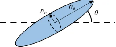
The SLM leverages the electro-optic properties of liquid crystals (LC) to effectively produce

a programmable phase mask. Depending on the orientation of a LC relative to incident light, the index of refraction is altered. The difference between the ordinary refractive

index,no, and the extraordinary refractive index,neis the birefringence and is the defining

optical characteristic of the LC.

∆n=ne−no (3.1)

By altering the bend angle of the crystal, the refractive index may be altered between no

andne. A diagram of a liquid crystal is shown in Fig. 3.3. The thickness of a liquid crystal

Figure 3.3: Diagram of liquid crystal showing the ordinary refractive index no, extraordi-nary refractive indexne, and bend angleθ.

CHAPTER 3. EXPERIMENTAL SYSTEM AND IMPLEMENTATION 32

phase change determined by

δ = 2π∆nd/λ (3.2)

where δ is the phase change in radians and λis the wavelength of light. On a diffractive

surface, a phase change of only 2πis required. As typical birefringence ranges from 0.05 to

0.45 [72] and considering the desired 2π phase change, the liquid crystal layer would need

minimum ranges in thickness from 1.4-13µm at a wavelength of 633 nm.

Liquid crystals align themselves with strong electric field, leading to their application

in electro-optical systems. For spatial light modulators, the electric field within the liquid

crystal is varied spatially to produce arbitrary phase patterns. A basic schematic for an SLM is shown in Fig. 3.4. A liquid crystal layer is sandwiched between two alignment

layers which are mechanically rubbed along a specific direction. The LC’s will self align

along this direction and only modify the phase of light which matches this polarization.

The front facing side has an anti-reflection coated transparent electrode which is connected

to an electrical ground. The back layer has an aluminum pixel array whose voltage can

be controlled individually by a CMOS chip. Increasing the voltage of a pixel increases the

electric field running perpendicularly between the pixel and the transparent electrode. The

greater the electric field, the greater the bend angle of the LCs. The aluminum pixel array also acts as a reflective surface for incident light. Light first pass through the transparent

electrode, then the LC layer, and then reflects off the pixel array, ultimately passing through

the LC layer twice [73].

The pixelated surface of the SLM leads to many challenges which must be overcome

to properly emulate a PSF engineered system. Some SLMs (not used in this thesis) have

an added dielectric reflective surface in front of the array which improves the diffractive

Figure 3.4: Cross section of the liquid crystal on silicon (LCOS) SLM.

Manufacturer Holoeye

Model Pluto GAEA-2

Pixel Pitch 8µm 3.74 µm

Resolution 1920x1080 4096x2160

Frame Rate 60 Hz 60 Hz

Fill Factor 93% 90%

Table 3.1: Specifications for spatial light modulators used in this work.

have effects from the pixelated surface.

In this work, two spatial light modulators were used from Holoeye Photonics [75]. The

specifications of these are shown in Tab. 3.1

3.2.2 Limitations of the SLM

The SLM provides a programmable pupil mask which allows for testing arbitrary phase

functions. Despite it’s versatility, the SLM has drawbacks that would not be present in a

static phase mask due to limited fill factor and diffraction efficiency. These drawbacks and

their solutions are discussed in this section.

Due to the phase quantization, spatial quantization, and dead regions of the SLM

between pixels, there is a zero order reflection from the SLM [76, 77]. In the case of beam

CHAPTER 3. EXPERIMENTAL SYSTEM AND IMPLEMENTATION 34

the optical axis. In the case of PSF engineered imaging, a ghost image of the scene is

present on top of the desired blurred image when the SLM is aligned with the optical axis. The effect is shown in Fig. 3.5. The image with a zero order artifact does not properly

resemble the desired imaging system.

Figure 3.5: Simulation illustrating the issue from zero order reflection of the SLM. a) Scene to be imaged. b) Desired image using axicon phase mask. c) Image with zero order ghost image.

Several methods have been previously studied for suppressing the zero order which

involve adding a corrective phase to the SLM. One method is adding a spherical wavefront

to the existing phase to move the focal plane of the diffractive light along the optical axis

[78]. This method greatly reduces the peak intensity of the zero order, but does not remove the unwanted light from the detector. As the image will also have a reduced intensity, this

method would not be effective. Another method would add a phase function which produces

a beam which destructively interferes with the zero order [79]. This method is not possible

with the Holoeye SLM which has a high speed flicker which would inconsistently eliminate

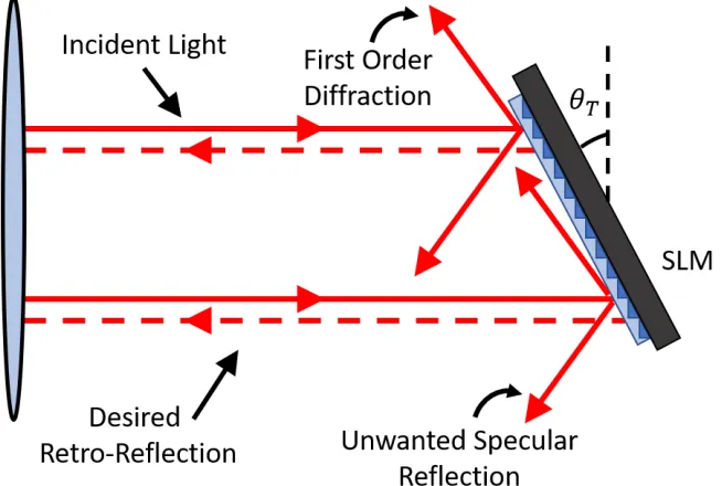
the zero order. The chosen method adds a tilt function to the SLM and rotates the angle

of the SLM to retro reflect the diffracted light while deflecting the zero order away from the

this work, a sawtooth function with period of 4 SLM pixels is used requiring a tilt angle of

θt= 2.43o tilt of the SLM to retro-reflect the desired light. The deflected zero-order image is blocked by the razor blade at an intermediate image as shown in Fig. 3.1.

Figure 3.6: SLM configuration with sawtooth phase function addressed to SLM and the SLM tilted to retro-reflect desired diffraction pattern. The angle θt is exaggerated in the figure with a value of 2.6o used in experiment.

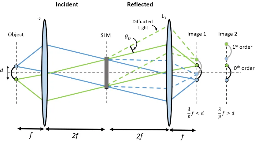
SLM is limited in field of view due to the pixelation of the SLM as reflected light is

diffracted into multiple orders. These multiple orders form multiple images of the scene

as shown in the ray trace in Fig. 3.7. The object of length d is brought to a distance by

lens L3 with focal length f. Light is reflected off the SLM and is diffracted into multiple

diffractive orders separated by angleθD =λ/pwherep is the pixel pitch of the SLM. The

light passes throughL3 again and forms an image of the object. Because of the diffractive

CHAPTER 3. EXPERIMENTAL SYSTEM AND IMPLEMENTATION 36

will overlap with one another. Because of this, the system must limit the field of view in

order to achieve f λ/p > d. In addition, because of the zero order light, the desired image must fit between two diffractive orders with the desired image fitting in between. Thus,

the intermediate object size a focal length in front of L3 must fulfill d < f λ/2p. As the

extended PSF will enlarge the image, the constraints are even tighter, but is dependent on

the extent of the PSF. This limit may be enforced using an aperture at the intermediate

image beforeL3.

Figure 3.7: Ray trace from a selected region of the experimental setup. Whenλf /p < d, there is overlap in the image plane between the subsequent diffractive orders.

Additional issues occur due to a duty cycle of the SLM. The SLM is advertised with a

refresh rate of 60 Hz. To analyze any effects the refresh rate may have on testing a static

phase function, a high speed Edgertronic SC1 record is used in lieu of the CCD in Fig. 3.1.

applied to the SLM to separate the zero order for the diffracted light. A duty cycle of

50% was found where the liquid crystals are in a relaxed state leaving only the zero order diffraction for 50% of the time. The on state, off state, and a line profile as a function of

time are shown in Fig. 3.8. In the line profile, a flicker can be seen where the intensity of the

desired light is oscillating. The oscillation appear consistent and does not affect imaging

as long as an integer number of periods of the duty are recorded in a single exposure.

a

20 60 100

x (pixel)

50

100

150

200

250

300

350

y (pixel)

b

20 60 100

x (pixel)

c

0 0.1 0.2 0.3 0.4

Time (s)

CHAPTER 3. EXPERIMENTAL SYSTEM AND IMPLEMENTATION 38

SLM’s typically contain surface errors which leads to wavefront errors and aberrations

in the imaging system [76, 77]. The PSF of the experimental system including the Holoeye GAEA SLM was recorded by imaging the laser spot in Fig. 3.1 alone with only the tilted

phase function on the SLM. The resulting aberrated PSF is shown in Fig. 3.9a. The

aberration was verified to be caused by the SLM by replacing the SLM with a flat mirror,

resulting in a near diffraction limited PSF. The aberrations will affect the OTF of the

system and lead to degradation in the reconstructions. Luckily, if the phase function is

known, the wavefront may be corrected using the SLM itself. As an alternative to using

a wavefront sensor, a stochastic parallel gradient descent (SPGD) algorithm is used to

optimize the PSF and correct aberrations [81, 82]. A random phase perturbation with a

maximum phase of about a quarter of a wave is added to the SLM to create a candidate phase correction using a basis of 14 Zernike polynomials (skipping piston). An image of

the laser spot is recorded and the sharpness is calculated as

Sharpness=X[I(x, y)2]/[XI(x, y)]2 (3.3)

where I are the intensity values of the image in counts. If the sharpness of the PSF

increases, then the candidate phase is retained and the same perturbation is added again.

If the sharpness is reduced, a new random perturbation is added to the current phase of the

SLM. The process is repeated until the PSF is satisfactory. The algorithm was tested using

the Holoeye GAEA SLM for 2000 iterations. The resulting corrected PSF and wavefront

correction is shown in Fig. 3.9b and 3.9c.

In experiment, the phase function of applied to the SLM (ΦSLM[x, y]) is the sum of the tilt function (ΦT ilt[x, y]), wavefront correction (ΦCorr[x, y]), and the desired phase function

Figure 3.9: a) The experimentally recorded PSF aberrated by the surface errors of the SLM. b) The experimentally recorded PSF after the SPGD algorithm. c) The phase function for correcting the SLM wavefront error.

experiment, the reflected wavefront emulates just the desired phase function.

Figure 3.10: Sum of tilt correction, aberration correction, and desired phase functions to produce phase on SLM. The sum creates the desired phase function in experiment.

3.3

Experimental Validation

An experiment is performed to observe the performance of the phase masks from Eq. 1.14

CHAPTER 3. EXPERIMENTAL SYSTEM AND IMPLEMENTATION 40

function are recorded and averaged to be treated as the diffraction limited imaging

perfor-mance. The same is repeated with the desired phase function added to the SLM. These images represent the PSF of the system.

The experiment is first performed with the axicon, vortex, and cubic phase functions

witha= 40, b= 15, andm= 20 as these each provide the same theoretical laser

suppres-sion of 0.02. The phase patterns, along with their experimental and theoretical PSF’s and

MTF’s, are shown in Fig 3.11.

While the expected laser suppression is 0.02, the measured suppression using the images

from Fig. 3.11 varied and are shown in Tab. 3.2.

Vortex Axicon Cubic 0o Cubic 45o

0.0216 0.0155 0.0175 0.0184

Table 3.2: Measured laser suppression. See peak intensities of Fig. 3.11 (k-o).

The target used in the experiment is a transmissive Air Force bar target. The target

is rear illuminated by a diffuse halogen lamp and filtered by a laser line filter to ensure

quasi-monochromatic light as the SLM is wavelength sensitive. The target and laser are

imaged simultaneously with each of the phase functions along with the sawtooth function.

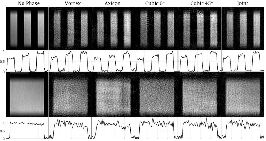
The resulting images are deconvolved with their respective measured PSF’s.

The detected and restored results are shown in Fig. 3.12. The images are displayed on a log scale to show faint noise artifacts that are difficult to see. Fig. 3.12 (a) and (f)

are the detected and restored images of the no phase case and represent the peak imaging

capabilities of the system. The no phase detected image was deconvolved to provide a fair

comparison for each of the modulated phases cases. The vortex and axicon cases show

ringing artifacts around the bars and are more prevalent around the restored laser spot.

CHAPTER 3. EXPERIMENTAL SYSTEM AND IMPLEMENTATION 42

cubic cases are much smaller and have less of an effect on the image. There also appears

to be less background noise which can be observed by looking at the uniformity of the bars and of the dark regions of the images. In terms of target resolution, there is no obvious

difference between the images qualitatively.

Figure 3.12: Experimentally recorded images using a) no phase, b) vortex, c) axicon, d) cubic, and e) rotated cubic masks. Corresponding restored images (f-j) and joint deconvo-lution (k). Images are gamma corrected to aid in viewing artifacts in the dark regions of the images and around the laser spot.

The vortex and axicon detected images and PSF’s were combined to create a joint

restoration using Eq. 2.26. The resulting image is shown in Fig. 3.12 k. While there are

more artifacts around the laser spot, there are much fewer artifacts around the bars and in the dark regions of the image. The artifacts around the laser spot show that there may be

noise artifacts in the coherent light not accounted for. The dampening parameter,γ(ξx, ξy)

is also much smaller than 1/SN R(ξx, ξy) for both the vortex and axicon case which leads

to a much brighter laser spot for the joint reconstruction. The intensity of the artifacts

versus the peak brightness of the laser spot is lower for that of the joint reconstruction

then it is for the vortex or axicon.

comparison of each mask’s performance. Observing the images, both the resolution of the

system and the added noise are important measures for the system. The General Image Quality Equation (GIQE) seeks to combine these metrics into a single quantity [61] with

GIQE =c1+c2×log10(RER/GSD)−c3×H−G/SN R where c1,c2, and c3 are scalar

coefficients, RER is the relative edge response, GSD is the distance between samples in

the scene,H is the edge overshoot andGis the noise gain. This metric relies on subjective

testing and was not intended for PSF’s whose performance varies depending on the angle

of the edge. In this report, the edge response and noise gain are presented separately.

To quantify the system resolution, the relative edge response is measured. Using the

line profile of the bars from Fig. 3.13, the maximum slope of the right most edge is taken.

The relative edge response is then calculated as the slope for the modulated cases divided by the unmodulated case. The value is expected to be between 0 and 1, with 0 having

the bars blurred uniformly over the image and 1 a perfect reconstruction of the diffraction

limited image. To quantify the noise gain, an RMS error was measured. Using the area of

the square from Fig. 3.13, the RMS error is calculated as

Noise Gain =

q_X

(I−1)2/N (3.4)

where I is the intensity at a given pixel and N area the number pixels in the are of the

square. The error of each mask was divided by the error of the unmodulated case. This

value is expected to be greater than 1 and provides a measure of how much greater the

noise is for this system than the diffraction limited system. A larger value represents a

worse image with more noise. The edge response and noise gain are shown in Fig. 3.14. The average line profile of the bars and a line profile of the square are both shown in

CHAPTER 3. EXPERIMENTAL SYSTEM AND IMPLEMENTATION 44

Figure 3.13: Same as Fig. 3.12, zoomed view of upper right hand bars (top) and middle left solid square (bottom), along with corresponding normalize line profiles.

As expected, the cubic phase mask, which has an MTF that performs best along the

horizontal and vertical edges of the bar target, produces the greatest edge response. The

vortex, rotated cubic, and the joint case each perform similarly. Each of the vortex, axicon,

and cubics have similar noise gain. The vortex and axicon, however, will produce greater

low frequency noise which is more prevalent to a human observer. The noise is apparent

in the line profiles for the squares shown in Fig. 3.13. The joint case produces the lowest

noise gain which supports the new deconvolution method for removing nulls in the MTF.

3.4

Summary

In this chapter, an experimental testbed was designed to validate the theoretic imaging

Figure 3.14: The relative edge response and noise gain measurements with each mask, showing improved noise suppression in the joint case.

powerful laser source using a beam splitter. The pupil with an arbitrary phase function

was tested using a phase-only SLM. Challenges associated with the SLM which would not

be present in the theoretic system including zero-order diffraction, limited field of view,

and added aberrations were discussed and overcome.

The experimental setup was implemented to image a resolution bar target with the

previously know phase functions: axicon, cubic, and vortex. The cubic was shown to

pro-vide the greatest imaging fidelity with the lowest noise gain giving epro-vidence an odd phase

function is advantageous over an even one. Exposures from the axicon and vortex phase function were combined through a joint deconvolution operation, allowing for their

respec-tive nulls to be compensated by one another. The result was a significant improvement in

noise gain over each of the individual reconstructions.

CHAPTER 3. EXPERIMENTAL SYSTEM AND IMPLEMENTATION 46

providing the expected PSFs and blurred images. Each reconstructions resulted in images

with suitable fidelity. Suffice to say that for each of the images, it is the goal to improve upon the performance of these masks either in significantly lower LSRor a high imaging

Pupil Phase Optimization

Using knowledge of PSF engineering, an optimal phase mask is sought which maximizes

the post-processed imaging fidelity for a fixedLSR. Using the integrated Strehl ratio as a

quantitative metric of image quality, numeric and analytic approaches are taken to produce

a desired phase mask. Simple techniques are not sufficient for optimizing the phase mask.

Consider a basis set consisting of:

Φ1(r, θ) =v1×2π

r

Rcos

3_{[θ] (4.1a)}

Φ2(r, θ) =v2×2π

r

Rcos

5_{[θ] (4.1b)}

where v1 and v4 are scalar constants, r and θ are the radial and azimuthal coordinates,

and R is the aperture radius. The values for Strehl and LSR can then be calculated for

the pupil function exp[i(Φ1(r, θ) + Φ2(r, θ))] and in turn the ratio Strehl/LSR may be

calculated. The values forStrehl/LSRare shown as a function ofv1 and v2 in Fig. 4.1.

This “topology” map forStrehl/LSRshows a peak value for the basis set atv1 = 17.4

CHAPTER 4. PUPIL PHASE OPTIMIZATION 48

Strehl/LSR

-20 -10 0 10 20

v

1

-20

-15

-10

-5

0

v

1 1.5 2 2.5 3 3.5 4

Figure 4.1: The value for the ratioStrehl/LSRas a function ofv1 and v2 given the phase

and v2 = −14.8. Because of the complexity of the topology map, numeric algorithms

which rely on the calc