Design a PID controller with missing packets in a networked servo-system

(1)

University of Southern Queensland

Faculty of Engineering and Surveying

Design a PID Controller with Missing Packets

in a Networked Servo-System

A dissertation submitted by

Sarang Ghude

In the fulfillment of requirements of

Course ENG8002 Project and Dissertation

towards the degree of

(2)

Abstract

Networked Control Systems (NCS) are defined as the systems in which a feedback control loop is implemented through a network. The networks employed for this task are based on a range of protocols. The data communicated through the network often face network congestions or collisions resulting in the loss of data carrying packets. This can impose a serious problem for the stability of the networked control systems. In this project, one such problem is studied, “Design of a PID controller with missing packets in a networked servo-system”. The controller under consideration is a discrete PID controller and the packets carrying error signals in a succession are considered missing.

(3)

(4)

CERTIFICATE

I certify that the ideas, designs and experimental work, results, analyses and conclusions set out in this dissertation are entirely my own effort, except where otherwise indicated and acknowledged.

I further certify that the work is original and has not been previously submitted for assessment in any other course or institution, except where specifically stated.

Sarang Ghude

Student Number: w0036313

Signature___________________

(5)

Acknowledgement

First, I would like to express my sincerest gratitude to Dr. Paul Wen for his valuable guidance, help and motivation throughout the conduct of this project without which completion of this project would have been a difficult task.

I would like to extend a special thanks to Dr. Tony Ahfock for finding some time for me in his busy schedule and contribution of his ideas about different aspects of control systems.

I am thankful to Dr. John Billingsley for his guidance and teaching in Robotics and Machine Vision course, which boosted my interest towards control theory and robotics.

Also, guidance from Dr. John Leis about research as a career proved very fruitful and a driving force behind completion of this project.

I am deeply grateful to Mr. Nils Uhlenbruch, for his valuable suggestions. I found discussions with him highly informative and beneficial. Sincere thanks would also go to Janice Swannell for proof reading this dissertation.

(6)

List of Figures

Figure 2.1 Hierarchical Structure of Networked Control systems……… 8

Figure 2.2 Direct Structure of Networked Control Systems……….. 8

Figure 2.3 Network Hierarchy………... 9

Figure 2.4 Token Bus Topology……… 12

Figure 2.5 Delays in Networked Control Systems……… 13

Figure 2.6 Time Components in a Source Node to Destination Delays……… 14

Figure 3.1 Position Control System………... 20

Figure 3.2a Time Constant………... 20

Figure 3.2b Integrator………... 20

Figure 3.3 Servo-System Response……… 22

Figure 3.4 Typical PID Response………... 24

Figure 3.5 Block Diagram of PID Controller and Motor………... 25

Figure 3.6 Practical PID Arrangements………... 25

Figure 3.7 Practical PID Response………... 26

Figure 4.1 Sampling……….... 29

Figure 4.2 Digitization……… 29

Figure 4.3 Bode Plot of the Plant……… 31

Figure 4.4 Discrete System Response with T=0.005 seconds……… 32

Figure 4.5 System Components for Optimization……….. 33

(10)

[image:10.595.145.540.48.392.2]

Figure 4.7 Output of C Program Showing Error Sum……… 35

Figure 4.8 Output of C Program with q = 0.2……… ₁ 36 Figure 4.9 Output of C Program with q =0.33………... 1 36 Figure 4.10 Output of C Program with q =0.262………. ₁ 36 Figure 4.11 System Response with New Controller Parameters……….. 37

Figure 4.12 System Response with Tuned Controller Parameters………... 38

Figure 5.1 Networked Model of the Servo-System……… 41

Figure 5.2 The Ethernet Frame/Packet Format………... 42

Figure 5.3 Tuned PID Response of the System……….. 44

Figure 5.4 System Response with e(k-2) when e(k) is missing……….. 45

Figure 5.5 System Response with e(k-1) Missing and Previous PID Parameters Values………. 47

Figure 5.6 System Response with e(k-1) Missing and New PID Parameters………. 48

(11)

List of Tables

Table 5.1 Comparison of the system responses with missing packets…………. 50

(12)

Chapter 1

Introduction

Networked Control Systems (NCS) are defined as the systems in which computer networks are used as paths. In networked control systems communication of data from sensor to controller or control signal from controller to actuator, occur through communication networks. In Networked Control Systems, the data are communicated in the form of packets. PID controllers are widely used controllers in the field of control systems because of their fantastic performance. It gives the combined effect of Proportional, Integral and Derivative controllers, so the system response is improved significantly.

(13)

1.1

Previous work

In (Wei Zhang 2001), the stability of the networked control systems with network induced delays is analyzed using ‘Hybrid Systems Stability Analysis Technique’ and the stability regions. Hybrid systems are continuous-discrete systems whereas stability regions are plotted with respect to the sampling rate and the network delay. The network delays are considered constant. It is mentioned that the network-induced delays occur when the data is exchanged among different nodes of a network. It says that depending on the Medium Access Control protocol of the network, these delays can be constant, time varying or random. In the analysis of the stability of the system with network delays, cases with delay less than one sampling period and delays longer than one sampling period are stated. The compensation methods for network-induced delays are also described.

In (Gregory C. Walsh 1999), Try-Once-Discard (TOD) network protocol is introduced. In this protocol, the node with the greatest weighted error from the last reported value wins the competition for the resource but if a data packet fails to win the competition for network access, it is discarded and new data is used next time. It introduces Maximum Allowable Transfer Interval (MATI) that is the time limit set to use the network resources. It gives the analytical proof of the global stability for a networked control system with general multiple packets transmission. It also gives global stability condition for one packet transmission problem.

(14)

In (Pohjola 2006), a PID controller is designed for the networked control system. In this thesis, there are examples of Time varying systems such as transport belt, tank pipe etc. The PID controller tuning is carried out by Ziegler Nichols method, Internal Model Control and by Gain scheduling. The optimization is done by cost function that is performance criterion such as IAE, ITAE etc. In this case, optimization is done with different types of delays such as constant delay, random delay, sinusoidal delay, state delay etc. These results were checked on MoCoNet system developed at the Helsinki University of Technology.

In (Raji 1994), it is stated that data networks use large data packets and relatively infrequent transmission rates, with high data rates to support the transmission of large data files. Control networks on the other hand are supposed to shuttle countless small but frequent packets among a relatively large set of nodes. In this paper, it is mentioned that the data networks and control networks can work together. This paper contains discussion about data network topologies. It says that, these can be used for control networks as well. A chart showing comparison of different distributed control media based on characteristics such as data rate, node cost installation cost etc is mentioned. It further says that, PID algorithms usually demand good response time. A figure shows OSI layers of network, typical tasks assigned to it and corresponding requirements of control networking. At the end a detailed comparison of the different control networks based on various characteristics is given.

(15)

1.2

Objectives

The main objective of this project is to design and tune a PID controller with missing packets in a networked system and then compare the output responses. The discrete PID controller is going to be used and the packets that would be considered as missing include packets carrying error terms e(k), e(k-1) and e(k-2). The first list of objectives is given in appendix A. The revised version of the list of objectives can be outlined as follows

1. Research the Networked Control Systems to get an overview of the networked systems such as their structures, networks, control methods etc.

2. Study the servo–system model and find out the transfer function.

3. Add the PID controller to the system and check out the system response.

4. Find out the discrete transfer function of the digitized system.

5. Add a Discrete PID controller and check the response.

6. Tune the PID controller with Steepest Descent Gradient Method.

7. Propose a networked model for the given servo-system.

8. Find out details about the Packet formation and the reasons for Packet loss.

9. Find the system response with missing e(k) and tune the controller (if required)

10. Find the system response with missing e(k-1) and tune the controller (if required)

11. Find out the system response with missing e(k-2) and tune the controller (if required)

(16)

1.3 Methodology

The aim of this project is to design and tune a discrete PID controller with missing packets in a networked servo-system. Networked control systems are overviewed to gain the familiarity with their structures, control networks and control methodologies used. The system or plant is a mechanical unit hosting a DC motor, from an analogue servo system by Feedback Instruments Ltd, UK. Therefore, there is a transition from analogue system to digital system then to a networked system. As an analogue system, given system is mathematically modeled. It is important to check the stability of the system, which is done by using Routh-Hurwitz criterion. The practical PID controller response is taken to verify the performance of the controller. As a digital system, derivation of the discrete mathematical model of the system is important because in a digital environment continuous plants are considered with a Zero-Order-Hold system. A discrete PID controller is used and tuned. The Steepest Descent Gradient Method is a mathematical approximation method that is used for tuning of PID controllers. This method involved complicated and laborious calculations so a computer program is developed to speed up the process. A networked model for the system is proposed with the use of Ethernet as a communication network. The packet formation in Ethernet and reasons for their loss are identified. The system responses with missing packets carrying error samples e(k), e(k-1) and e(k-2) are taken. These responses are then compared and analyzed.

1.4 Thesis Structure

Chapter 2

This chapter is an overview of the networked control systems. At start, the structures of the networked control systems are explained. Then, control networks and protocols followed by the delays associated with the systems are discussed. At the end, different control methodologies are reviewed.

Chapter 3

(17)

Chapter 4

In this chapter, digitization process is explained. Then, the discrete transfer function of the system is derived and the system response is checked. After that, a discrete PID controller is added to the system and it is tuned by Steepest Descent Gradient method.

Chapter 5

In this chapter, networked model of the servo-system is proposed. Then, Ethernet and its packet structure are discussed. The reasons for packet loss are explained in the following section. Then, system responses with missing e(k), e(k-1) and e(k-2) are found and at last the obtained results are compared and analyzed.

Chapter 6

This chapter contains the conclusion and directions for the future work.

Appendices

The appendices attached include, A) Project Specifications.

B) Simulink Models. C) The C program code.

(18)

Chapter 2

Networked Control Systems: An Overview

This project deals with the issue of missing samples, which is an important part of networked control. In this chapter, the networked control system is reviewed. Here, information is gathered from different sources. At the start, the structures of networked control systems are discussed then different network protocols and networks based on them are examined. These protocols are implemented at the medium access control sublayer and they control the information transmission.(Y Koren 1996) Then the delays in the networks and their time components are discussed. These delays occur in data transmission mainly. Lastly, there is a brief introduction to some control methodologies, which are developed so far to give better control performance while marinating stability of the system.

2.1 Structures of NCS

(19)

[image:19.595.154.497.82.229.2]

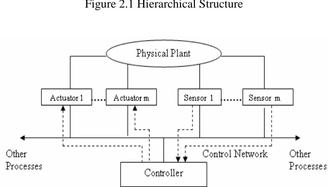
Figure 2.1 Hierarchical Structure

Figure 2.2 Direct Structure reproduced from (Wei Zhang 2001)

2.1.1 Hierarchical Structure

[image:19.595.162.496.247.435.2]

(20)

networked closed loop system. As shown in figure 2.1, the main controller can be designed to handle multiple networked loops, for several remote systems.(Yodyium Tipsuwan 2003). As the hierarchical structure is modular, its configuration is easy.

2.1.2 Direct Structure

The direct structure is shown in figure 2.2. In the direct structure of NCS, the controller is connected to actuators and sensors of a plant through the network. The connecting network here is the data network and forms a direct link between plant and the controller. The plant and the controller could be located at different locations. The system operation is simple. The controller computes the control signal and encloses it in a frame or packet. This packet is sent to the plant through the network. The plant then sends the system output back to the controller in a packet or frame. (Yodyium Tipsuwan 2003) An advantage of direct structure is that data is exchanged directly between controller and system components. Hence, the controller can observe and process every measurement sent to it.(Mo-Yuen Chow 2001)

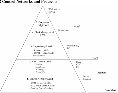
[image:20.595.129.543.399.724.2]

2.2 Control Networks and Protocols

(21)

There are different types of networks, applied at different levels of the system for successful implementation of the networked control. Figure 2.3, shows a general hierarchy of different levels and the networks that can be used. Level 1, is the root level where controllers, sensors and actuators are connected through a network Examples of networks and protocols at this level include CAN, DeviceNet, SDS, ASI, Bitbus, Interbus, P-Net, Seriplex, Sercos Interface. It is called Sensorbus. Level 2 is cell control level. At this level, control cells such as PLC, CNC, and PC are connected through the network. Examples Profibus, LonWorks, WorldFip, ControlNet etc. It is called Fieldbus. Level 3 is the Supervisory level, which mainly hosts a network of computers. It is called as LAN (Local Area Network). Examples of networks and protocols include Ethernet, MAP, TCP/IP, Ethernet/IP, and Modbus/TCP. Level four and five are management levels in which mainly workstations are connected in the network. These could be in a single building or different locations.

(22)

2.2.1 CSMA/CD

CSMA/CD stands for Carrier Sense Multiple Access with Collision Detection. This protocol is specified in IEEE 802.3 networks standards. From Leis, (2005), Tanenbaum, (1996), this protocol can be explained as follows. In this protocol when a node wants to transmit the data it listens for the availability of the network. If the network is busy, the node waits until it goes idle. Otherwise, it transmits immediately. After that, each node has to listen for the detection of data collision. The occurrence of a collision must be signaled to all other nodes on the network to signify that a problem has occurred. This is done by the transmitting node continuing to transmit for 32 to 48 bits to enforce collision. When two or more stations simultaneously begin data transmission on an idle network, the data will collide. All the nodes involved in collision then stop transmission and wait for a random amount of time before making an attempt of transmission. This random time can be calculated by Truncated Binary Exponential Backoff algorithm. The waiting time before making transmission attempt is chosen randomly between zero and 2n−1 slot times where n is the number of nth collision detected by the node. The slot time is the time taken for the round trip transmission. The waiting period is set to 1023 slots after occurrence of 10 collisions. After 16 collisions, the failure is reported back to the node. The control network based on this protocol is Ethernet.

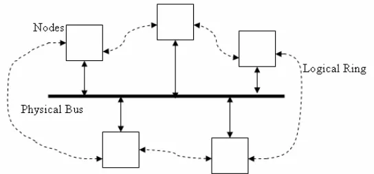
2.2.2 Token Bus or Ring

(23)

[image:23.595.201.473.121.248.2]

Field Bus Profibus, Manufacturing Automation Protocol (MAP), ContolNet, Fiber Distributed Data Interface (FDDI).

Figure 2.4 Token Bus Topology (Leis 2005), p5.8

2.2.3 CAN (CSMA/AMP)

(24)

2.3 Delays in Networked Control System

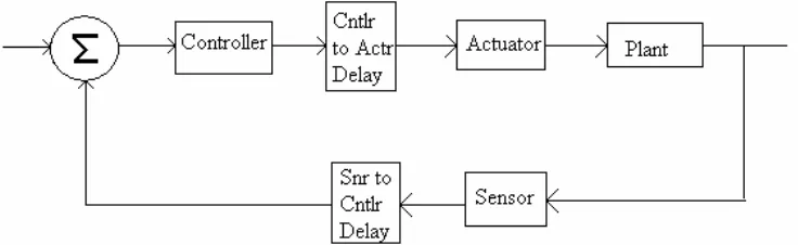
[image:24.595.144.512.340.453.2]

In a networked control, generated sensor data is immediately stored at the sensor terminals transmitter buffer. It waits there to be transmitted as a message through the network. After transmission, the sensor data is received by the controller and is kept in the receiver buffer until the next sampling instant of the controller. Then the data is processed and the resulting control signal is kept in the controller’s transmitter buffer. There it waits to be transmitted to the actuator terminal. Finally, after the arrival of the control signal at the actuator terminal, it immediately acts upon the plant. This is how the data communication and computational delays are induced in the networked control systems. Performance of Networked Control Systems can deteriorate because of these delays. Effects of delays can be overcome by setting up a long sampling period compared to these delays.

Figure 2.5 Delays in Networked Control System

Sensor to Controller Delay:

This delay is the time difference between the instant when controller starts computing the control signal and the instant when sensor reads the system output.

τSC =tCCS −tSR

Controller to Actuator Delay:

This delay is the time difference between the instant when controller completes

computing control signal and the time instant when actuator receives the control signal and starts processing it.

CA CFS AP

t t

(25)

Computational Delay in Controller:

This delay is the time taken by the controller to compute the control signal. That is time difference between the instant when it receives measurements from sensor and the instant when it completes the calculation of the signal.

CC CFS CCS

t t

τ = −

The sum of the above mentioned delays is called control delay (J. Nilsson 1998).

2.3.1 Time Components in Delays

Sensor to controller and controller to actuator delays are characterized by certain time delay components. According to Feng-Li Lian, (2001),

(2.1)

Where (T_scomp+T_scode) is the preprocessing time,

queue block

(T +T ) is the waiting time, (T_frame+T_prop)is the network time delay, (T_dcode+T_decomp)is the postprocessing time.

delay

T in equation 2.1 is the delay between two nodes for example sensor to controller or controller to actuator. The transmitting node acts as source and receiving node acts as a destination node. The communication between source and destination node takes place as follows

[image:25.595.145.509.571.688.2]

Figure 2.6 Time Components in a Source Node to Destination Node Delay (Lian 2001), p41

delay scomp scode queue block frame prop dcode decomp

(26)

• Preprocessing Time ( T_PREP): It is the time taken by the source node to compute the data from external environment and encode it into appropriate data format. The computation time is represented by T_scomp and the encoding time is represented byT_scode. Preprocessing time is dependant on software and hardware characteristics of the system.

• Waiting Time (T_WAIT): It is the time spent by the data in waiting for the network access. It is composed ofT_queue, time for which data waits in the buffer of the source node while previous messages in the queue are sent. Moreover,T_block is the time data must wait, once the source node is ready to send it. It includes the time of waiting while other nodes are sending their data and the time required to resend the data if collision occurs. It depends on network protocol and very important for the performance of network.

• Network Time (T_NETWORK): It is the time taken by the data to travel through the network. It involves frame timeT_FRAME, and the propagation timeT_PROP. Frame time is the time spent by the source in placing the data or frame on the network. Propagation time is the travel time of the data through actual network or physical media of the network. It depends on the speed of transmission and distance of the source node and the destination node.

2.3.2 Vacant Sampling

In Sensor to Controller or Controller to Actuator communication, if the source node transmits a data and due to data loss in between, the data does not arrive at the destination node before the occurrence of next sampling period. In this case, there is no new data or measurement to compute the next control signal, so the previous data or measurement is used to calculate the control signal. This is known as Vacant Sampling. For example, the sensor data y and k yk+1 reach the controllers receiver before and after

(27)

For this, buffer size of the controller receiver needs to be increased so that the delayed data can be used for data reconstruction instead of simply being overwritten.

(A. Ray 1988; Y. Halevi 1988)

2.3.3 Message Rejection

If at the destination node, two data messages arrive during the same sampling period, then the controller accepts the most recent data message and rejects the previous one. In other words if data messages say d and _k d_k₊₁ arrive at the destination node at the same sampling period k+1. Then d_k₊₁ will be accepted and d will be rejected. This is called _k

Message Rejection.(A. Ray 1988)

2.4 Control Methodologies in NCS

In a networked control system, a control method should provide stability along with better performance and control action, in presence of delays. These control methods are mainly designed according to network behaviors, network configurations and the ways of treating delays. Few such methods are compiled by (Yodyium Tipsuwan 2003). These methods are listed below.

1. Augmented deterministic discrete-time model methodology

This methodology deals with periodic delay network and with some modifications, it can be used to support non-identical sampling periods of a sensor and a controller. This method gives the necessary and sufficient condition for uniform asymptotic stability of networked systems with periodic delays.(A. Ray 1988)

2. Queuing methodology

(28)

this method, state prediction/control scheme is proposed. This scheme uses, knowledge of the amount of data in the queue to enhance the prediction of the state.(H Chan 1995)

3. Optimal Stochastic Control Methodology

In this methodology, effects of random network delays are treated as Linear-Quadratic-Gaussian (LQG) problem. It assumesτ <T. It takes into account past information of output as well as input along with past information of delays. It gives the condition for stochastic stability of the closed loop system.

4. Perturbation Methodology

In this methodology, non-linear and perturbation theory is used to formulate network delay effects as the vanishing perturbation of a continuous-time system under the assumption that there is no observation noise. It requires small sampling time so that the system can be approximated as continuous plant.

5. Sampling Time Scheduling Methodology

As the name suggests, in this methodology a sampling period is selected in such a way that control performance of the networked control systems is not affected significantly and the system remains stable. This method can be applied to multiple networked control systems.

6. Robust Control Methodology

(29)

7. Fuzzy Logic Modulation Methodology

Here, PI controller gains are externally updated at the controller output with respect to the system output error caused by the network delays. Therefore, the controller needs not to be redesigned, modified or for use on a networked environment. A fuzzy logic modulator is used to modify the controller output.

8. Event Based Methodology

This methodology can be used for hierarchical as well as direct structures. It uses system motion as the reference. System motion has to be a non-decreasing function of time to guarantee the system stability.

9. End-user control adaptation methodology

In this methodology, controller parameters such as controller gain etc are adapted with respect to current network’s traffic conditions or its quality of service. This method assumes that controller and remote systems can measure network traffic conditions.

2.5 Chapter Summary

(30)

Chapter 3

Servo-System Model and PID Control

It is from a general methodology of a control system design that a system transfer function from the given model of the system is first derived. The stability of the system is then checked. After that, a system response is plotted and the next stage is controller design and the final response of the system. In this chapter, almost the same methodology is followed. First the system model is introduced, then derivation of its transfer function. System stability is checked with the Routh-Hurwitz criterion. A system response is checked with Simulink. For better system performance, the PID controller and its properties are explored. A complete system response is checked with actual circuit components.

3.1 System Model

(31)

Thus, a servo-system hosts a mechanism to provide control action that is controller designing can be done on a servo unit. This servo-unit is then connected to the plant. In the present case, servo unit is the analogue unit and mechanical unit is the plant. When position control is considered, the system block design for position loop is given as fig 3.1.

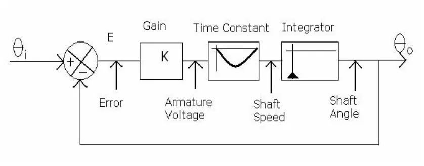
Figure 3.1 Position Control System

(Manual 33-002, feedback systems ltd. UK), p4-14-19

The motor characteristics can be expressed by the time constant (relating armature voltage and speed) followed by an integration (relating speed and output shaft position).

The Time Constant Circuit is a RC circuit and voltage is measured across the capacitor where 1

CR

ω =

And

ω

is frequency in rad/sec. R C 1

V ₁ V ₂ V ₁ R ₁ V ₂

[image:31.595.113.532.163.327.2]

Op-Amp

Figure 3.2 a) Time Constant b) Integrator

(Manual 33-002, Feedback systems ltd. UK), a) p 4-14-7 b) p4-14-11 In case of Integrator, the transfer magnitude is unity for 1

CR

ω =

Therefore 2 1

1 2

V

(32)

3.2 System Transfer Function

From the frequency domain block diagram of the system, there are four components Gain, Time Constant and Integrator and a feedback. Thus to find the transfer function of the system, Laplace transform of these three blocks will be taken and then block reduction techniques applied.

For Gain, The Laplace transform will be the amount of Gain only because in case of gain there is Laplace transform of output equal to gain times Laplace transform of input.

For Time Constant, since it is a RC circuit Laplace Transform comes 1 1

RCs+

For Integrator the Laplace transform is 1

i

T s where T =0.04 so, we get

1 0.04s Moreover, the Laplace transform of feedback will be unity

Thus for the System Transfer Function

Transfer Function ( )

1 ( ) ( )

G s TF

G s H s

=

+ ⋅

Where ( )G s =L Gain L Time Constat{ }⋅ { }⋅L Integrator{ } Let K be the gain. So finally

₂

0.04 0.04

K TF

RCs s K

=

× + +

Substituting values of K, R, and C as 1, 200K and 1 µF respectively in above equation

₂ 1

0.008 0.04 1

Transfer Function

s s

=

+ + --- (3.1)

3.3 System Stability

(33)

coefficients of the characteristic equation. Hurwitz criterion describes the asymptotic stability of the system.

3.3.1 Routh-Hurwitz Criterion

The system stability was tested using Routh-Hurwitz criterion. Equation 3.1 can be written as ₂ 125 5 125 Transfer Function s s =

+ + --- (3.2) So, the characteristic equation is s2+ +5s 125=0 --- (3.3) As per (Ogata 2002) the necessary but not sufficient condition for stability is that the coefficients of characteristic equation all be present and have a positive sign.

In equation 3.3, the last term is 125, that means any zero-root is absent and as all the coefficients are positive, it shows absolute stability

The Routh Array can be tabulated as follows

It shows that all the terms in the first column are positive that means all the roots are in left half of s-plane.

Now using Hurwitz stability criterion

As the determinant value is 625, which is greater than zero, the system is asymptotically stable.

3.4 System Response

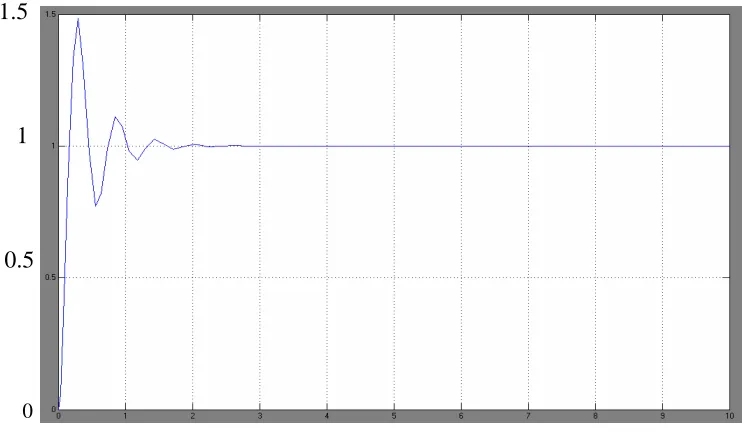
For the given system, a simulated response was checked with a step input, and using Simulink. The response found was as in figure 3.3 on next page. This shows some oscillations, initial overshoot and little longer settling time. It indicates need of a controller, which will give less overshoot, less or no oscillations and quicker settling time. A PID controller, which is Proportional + Integral + Derivative controller, can be used for this purpose.

(34)

1.5

1

0.5

[image:34.595.122.496.59.276.2]

₀

Figure 3.3 Servo-System Response

3.5 PID Control

A PID controller gives combined effect of three controllers that is Proportional, Integral and Derivative. Hence, it is most widely used controller in the industry. According to Astrom K J (1995), PID controller, in the form known today, emerged in the period from 1915 to 1940. It can be implemented in different forms, as a stand-alone controller or as a part of direct digital control or hierarchical distributed process control system. It can be divided into two categories Analogue (continuous) or Digital (discrete) PID controller. After selection of PID controller, it needs to be adjusted or tuned in order to get the optimum performance. For tuning of a PID controller many tuning rules are proposed and are in use. As a PID controller is a combination of proportional, integral, and derivative controllers, the individual properties of each of these controllers should be examined. Here the properties are in terms of response to a step input.

3.5.1 Properties of P, I and D controllers

The properties of a P controller can be summarized as; in a P controller, the control action is directly proportional to the error term; the rise time of the response decreases; the overshoot increases; settling time faces a small change; and the steady state error decreases. It was observed, with high gain, number of oscillations was more and the maximum overshoot increased.

(35)

The properties of a I controller can be summarized as; in a I controller the control action is directly proportional to the accumulated error; the rise time of the response decreases; the overshoot and settling time increases; and the I controller eliminates the steady state error completely.

m t( )=K_i

∫

e t dt( )

The properties of a D controller can be summarized as; in a D controller, the control action is proportional to the rate of change of error; there is a small change in rise time; the overshoot and settling time decreases; and the steady state error experiences a small change.

m t( ) K_D de t( ) dt

=

3.5.2 Properties of a PID controller

When all three controllers are combined together as a PID, it exhibits properties as follows. These properties are in terms of response to a step input:

• The response has a quicker rise time. • It has fewer or no oscillations. • There is no steady state error.

Mathematically, m t( ) K e t_P ( ) K_i e t dt( ) K_d de t( ) dt

= +

∫

+ [image:35.595.179.476.530.725.2]

Graphically a typical PID response can be shown as,

(36)

3.6 Analogue PID controller and System Response

Working with an analogue system, the servo system has a circuitry where a PID controller can be designed or arranged. So, let us have a look at some of the characteristics of an analogue PID controller. Realization of an analogue PID controller is given in appendices. The transfer function of an analogue PID controller can be written as,

TFpid =

2

D P i

K s K s K s

+ +

[image:36.595.141.509.262.413.2]

--- (3.4) The block diagram of the system with a PID controller can be drawn as follows,

Figure 3.5 Block Diagram PID controller + Motor

After adding PID controller, combined transfer function of the system can be written as,

Tfsys =

2

3 2

125 125 125

(125 5) 125 125

D P i

K s K K

s K s K s K

+ +

+ + + +

To find the system response, values ofKP,KD,Ki are needed. These values are

dependant on the values of the circuit components. On the servo system actual circuit arrangement can be made as follows,

Figure 3.6 Practical PID arrangements

(Manual 33-002, feedback systems ltd. UK), p4-12-12

[image:36.595.164.484.595.697.2]

(37)

To get the required values, transfer function of above system was derived using voltage divider rule,

Vo Zf

Vin= −Zin

Then, the resulting equation was compared with the transfer function of analogue PID controller that is equation 3.4. And the values of K_P,K_D_,K_i were found as follows K_D =0.11, K_P =1.13, K_i =1.25

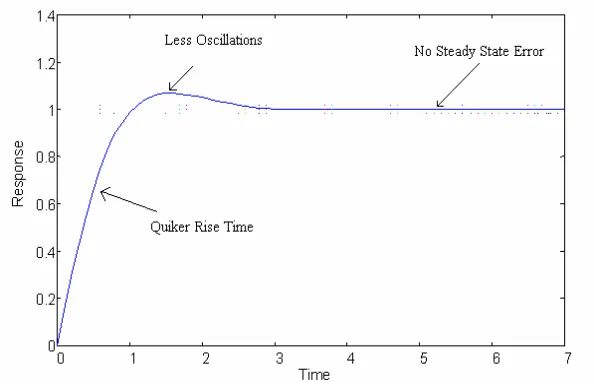
Using these values and Simulink software, the system response was checked and it was found as follows

1.4

1

0.6

[image:37.595.127.530.273.503.2]

₀

Figure 3.7 Practical PID response

(38)

3.7 Chapter Summary

(39)

Chapter 4

Digitization and PID controller Tuning

The concept of missing samples is associated with networked control of a system. To implement the networked control, the continuous system should be used in a digital environment. It can be done by digitization. In this chapter digitization and some important terms associated with it are explained. The system transfer function in z-domain using a discrete PID controller is derived. The minimum sampling period is found out using Bode plot. The systems simulated response in a digital environment is plotted. After that, the Steepest Descent Gradient tuning method is introduced and it is implemented in the current system. Lastly, the system response with tuned controller is checked.

4.1 Digitization

(40)

Sampling Frequency can be defined as a frequency at which a given signal is

sampled or in other words, it is a rate of sampling.

Sampling Period can be defined as the time interval between two successive

[image:40.595.116.539.159.290.2]

samples in a sampled signal.

Figure 4.1 Sampling [Lecture Notes]

Zero-Order Hold System, it is a system, which holds the continuous signal to

the last sampled value, till it gets a new sampling value through the sampling period. Graphically a digitization process can be shown as follows

Figure 4.2. Digitization (Gene F Franklin 1998), p58

4.2 Discrete System Transfer Function

When a digitized system is considered for the transfer function of the system, the plant is considered with the zero order hold system. And the plant transfer function is derived using formula,

G_HP( )z (1 z 1) {z G s( )}

s

−

= −

[image:40.595.119.536.418.566.2]

(41)

Using above formula and ( ) ₂125 5

G s

s s

=

+ the system plant transfer function is derived as

1 5 1 1 2

1 5 1

25 (1 ) 5(1 )

( )

(1 )(1 )

T

HP T

Tz e z z

G z

z e z

− − − −

− − −

− + −

=

− − --- (4.1)

where T is the sampling period.

With reference to figure 3.3, system transfer function is derived from the controller and plant transfer functions and unity step feedback loop. Thus, system transfer function can be written as,

( ) ( ) ( )

1 ( ) ( )

C HP

G z G z T z

G z G z

× =

+ × --- (4.2)

where G_C( )z is the transfer function of digital PID controller and,

1 2

0 1 2

1

( )

(1 )

C

q q z q z G z z − − − + + =

− --- (4.3)

The whole system transfer function using equations 4.1, 4.2 and 4.3,

1 2 1 5 1 1 2

0 1 2

1 1 5 1

1 2 1 5 1 1 2

0 1 2

1 1 5 1

( ) 25 (1 ) 5(1 )

( ) (1 ) (1 )(1 )

( )

( ) 25 (1 ) 5(1 )

( ) 1

(1 ) (1 )(1 )

T T T

T

q q z q z Tz e z z

C z z z e z

T z

q q z q z Tz e z z R z

z z e z

− − − − − − − − − − − − − − − − − − − − + + _× − + − − − − = = + + − + − + × − − − --- (4.4)

where T is the sampling period.

4.2.1 Finding Sampling Period (T)

(42)

[image:42.595.191.463.55.278.2]

Figure 4.3 Bode Plot of the plant ₂125 5

s + s

To find the sampling period, bode plot of the plant was found. Frequency corresponding to -3 dB magnitude is 12.8 rad/sec. This is the cut-off frequency. According to the sampling theorem, a continuous signal can be reconstructed from a sampled signal, if the original signal was sampled with a frequency higher than twice of cut-off frequency.

Therefore, sampling frequency

ω

s

≥

2

ω

c

and time interval

2

s

T

π

ω

=

According to our cut-off frequency 12.8 rad/sec, sampling frequency should be at least

ω

s = 33.6 rad/sec.

In that case time interval would be T = 0.19 sec.

4.3 Discrete System Response

To match the step response of a continuous PID controller with a discrete controller attention should be paid to some conditions, which are as follows,

q₀ >0, q₁≤ −q₀ and −(q₀+q₁)<q₂<q₀

with rectangular integration as mentioned in chapter 4 of (Dr. Paul Wen 2005) ₀ (1 d), ₁ (1 2 d )

i

T T T

q K q K

T T T

= + = − + − and ₂ KTd

q T

(43)

Thus from these equations the controller parameters are easily calculated, for which values of q q q₀, ₁, ₂ that can give better system response are needed.

The system can be modeled in Simulink. The Simulink model is given in the appendices. To start with the simulation values of q q q0, 1, 2 as 0.5, -0.5 and 0 are

assumed respectively. The system was simulated with sampling period T = 0.19 and it was found that the resulting signal has large samples. Thus, the sampling period was further reduced to 0.005. If the sampling period is further reduced then discrete nature of the signal is not visible. With 0.005 the sampling frequency 1256.64 rad/sec is achieved which satisfies the sampling theorem. The simulated system response with T=0.005 is shown in figure 4.3.

The response can be characterized as, a response with good rise time about half a second but with high overshoot around 1.35 and some oscillations. The settling time is also over 2 seconds.

1.4

1

0

Figure 4.4 Discrete System Response with T = 0.005 seconds The response characteristics are

(44)

4.4 PID Controller Tuning (Steepest Descent Gradient Method)

In this case, tuning of PID controller is basically, an optimization of q q q₀, ₁, ₂, which minimizes the error function of the system. For analysis of system error function, several mathematical techniques are available. According to (Dr. Paul Wen 2005), the type of mathematical analysis employed is dependant on the type of performance improvement desired. Basic system components for optimization are shown in the figure below

k

r

∑

e_k m_k c_k [image:44.595.141.506.224.339.2]

+ _

Figure 4.5 System Components for Optimization

Where Gc(z) and GHP(z) are the transfer functions of controller and plant represented by equations 4.3 and 4.1 respectively and,

m_k =q e₀ _k+q e₁ _k₋₁+q e₂ _k₋₂+m_k₋₁ --- (4.5)

e_k = −r_k c_k --- (4.6) Optimization of q q q₀, ₁, ₂ is done to minimize error function. Some functions that can

be used as performance criterion or error functions are as follows, 1.

∑

|e_k|, IAE, Integral Absolute Error.

2.

∑

k e| _k|, ITAE, Integral Time * Absolute Error. 3.

∑

ek2, Integral Squared Error.

4.

∑

(ek2 +

λ

mk2) Quadratic Performance Criterion. (Dr. Paul Wen 2005)

As per the Steepest Descent Gradient Method, a characteristic equation in terms of r_k

and c_kis derived by simplification and conversion of system transfer function in z-domain.

Then using one of the performance criterion or error functions listed above it is possible to get optimum values of q q q₀, ₁, ₂.

(45)

First values for q q_0, ₁ and q₂ are assumed, then the error function calculated. Then different values of q q_0, ₁ and q₂ are tried to get minimum value of the error function. To do this the value of q₀ is increased by a small step-size, keeping other two values constant.

Once a value for q₀ is fixed, this step is repeated for q₁ and q₂.

Figure 4.6 Steepest Descent Curve

As shown in the above figure, an initial assumption of q q q₀, ₁, ₂ is made starting at point 1 or 2 on the curve. In this case, depending on the point chosen, increasing or decreasing values of q₀ are taken by a small step size until minimum error point is reached. This is the new value of q₀. Keeping this value and q₂ the same procedure is repeated for q1 and then for q2.

A new value of q₀ is found by using formula ₀ ₀'

0 S q q q γ ∂ = ±

∆ ∂ --- (4.7)

whereγ =0.01,

(

0 1 2

) (

0 1 2

)

0

, , , ,

S q q q q S q q q S q q

δ

+ − ∂ =

∂ --- (4.8)

' 0

q Previous value of q₀ and

2 2 2

0 1 2

S S S

q q q

 _∂  _∂   _∂  ∆ =   +  +  ∂ ∂  ∂ 

  --- (4.9)

and S is the error function for example

0

| |

N k k

S k e

=

(46)

0 0 0 0 1 5

0 0 1 1 2

5 5

1 1 2 2 2 2

5

0 0 1

5 5

0 0 1

(1 5 ) ( ) 5 ( ) (25 10 5 ) ( 1)

( 25 5 25 10 5 ) ( 2)

( 25 5 25 10 ) ( 3) ( 25 5 ) ( 4)

(2 25 10 5 ) ( 1)

( 1 2 25 5 25 10

T

T T

T

T T

q C k q r k Tq q q r k

Tq e q Tq q q r k

Te q q Tq q r k Te q q r k e Tq q q c k

e Tq e q Tq

− − − − − − + = + − + − + − + + − + − + − + + − − + − − − + + − + − −

+ − − + − − + 1 2

5 5

1 1 2 2

5

2 2

5 ) ( 2)

( 25 5 25 10 ) ( 3)

(25 5 ) ( 4)

T T

T

q q c k e Te q q Tq q c k

Te q q c k

− −

−

− −

+ + − − + −

+ + −

4.5 Implementation of Steepest Descent Gradient Method

In this case, the characteristic equation from equation 4.4 was found to be

--- (4.7) Values of q q q were assumed as 0.5, -0.5, 0 respectively because according to ₀, ₁, ₂

Dr. Paul Wen (2005) at the start of minimization process, parameters should ensure a stable system and q₂ =0, q₀ =small and positive = - q₁can give the required parameters. After this, the next step was to calculate error signal ( )e k , using equation

4.6, ( )r k =1where k≥0and ( )c k (from equation 4.7). Then to find an error sum using

one of the performance criterion listed in section 4.4. To find this error sum number of samples (k) was taken in thousands, as the system simulation was checked for a few seconds. As k was in thousands, to make calculations quicker and faster a program in C was written. This program was written in such a way that it gave not only error sum but also the simplified equation for c(k) which keeps on changing with different set of values for q q q . The system response with the assumed values for ₀, ₁, ₂ q q q is ₀, ₁, ₂ shown in figure 4.3. To optimize the response, as per steepest descent gradient method, a new value of q was found by subtracting 0.01 (a step size calculated using equations ₀

4.7 to 4.9) from 0.5 keeping q q constant. The error sum using IAE performance ₁, ₂ criterion and the C program, was calculated and the output of the program was

(47)

The Error Sum value was too high and hence undesirable. Thus, the value of q was ₀

increased by 0.01, to 0.51 and then the error sum was calculated, it turned out to be 22.435197. It was further observed that with the increase in value of q , the error sum 0

value goes on decreasing. Hence value of q was kept constant to 0.5 and value of ₀ q ₁

was changed from -0.5. This time step size was 0.1 and it was added to -0.5. The error sum started decreasing till q reached to 0.2, and then at ₁ q₁ =0.33 the error sum increased. This showed that error sum was following the curve as shown in figure 4.5. After few trials and errors the minimum error point was found at 0.262.

Figure 4.8 Output of C program with q =0.2 ₁

Now q = - 0 q and 1 q2 =0can give the stable system. So, simulation was carried out with

(48)

1.4

1

0

Figure 4.11 System response with new controller parameters Comparison of figure 4.3 and figure 4.10 shows that, with new set of values of

0, 1, 2

q q q , the system response has improved.

The characteristics of this response can be listed as follows, Rise Time = 0.2833

Delay Time = 0.21 seconds Settling Time = 2.71 seconds Maximum Overshoot = 22%

It shows that the overshoot is less, number of oscillations has decreased. Thus, in search of better response, the values of q , ₀ q were further reduced and responses were ₁

(49)

1.4

1

0

Figure 4.12 System response with tuned controller parameters This shows that the controller is tuned with parameters q =0.06, ₀ q = -0.06 and ₁ q₂ =0 The characteristics of the graph can be stated as follows,

Rise Time = 1.12 seconds Delay Time = 0.588 seconds Settling Time = 2.294 seconds Maximum Overshoot = 0%

It shows that the desired characteristics are achieved. Though the rise time and the delay time have increased the settling, time has improved. Most important is the overshoot, with tuned controller there is neither overshoot nor oscillations.

4.6 Chapter Summery

(50)

(51)

Chapter 5

Missing Packets and PID Tuning

The issue of missing sample arises when the system involves networks for data or control signal communication. The original system in this project is an analogue system. Thus to deal with the issue of missing samples, a networked model for the servo system has been proposed. The structural model of the proposed system is discussed first. In digital environment and network, these feedback samples are encapsulated in different packets and these packets are communicated between nodes. Thus, this project is mainly about missing packets containing sample values. The Ethernet is discussed as a network for communication mainly focusing on packet formation in Ethernet. The packet losses are discussed next. Then, PID controller is designed and tuned with missing error signal e(k), followed by design and tuning of PID controller with missing e(k-1) and e(k-2) respectively. Lastly, all these PID responses are compared with the original system response.

5.1 Networked model of the system

(52)

[image:52.595.138.507.85.187.2]

Figure 5.1 Networked Model of the given System.

As in the hierarchical structure of a networked system, here two controllers are used. The first controller is the main controller, which would be used for calculation of control signal. The second controller is the local controller connected to the plant and the sensors. This controller would be responsible for retrieval of control signal from its digitized form, to convert it to the PWM signal and then to pass it to the plant. Sensors would measure the output of the plant and then send it to the local controller. The local controller would compare measurement with input signal. By this controller, the resulting error signal would be encapsulated to a data packet and transferred to the main controller via a computer network, for calculation of control signal. The main controller would then calculate the control signal using PID controller algorithm and send the control signal encapsulated in a data packet to the second or local controller. The main controller and the local controller would be considered as two separate nodes in the network. The computer network that could be used is Ethernet. To propose the networked version of the system, few assumptions were made and those are as follows,

♦ This system is one part of the large networked system. So, the network is used by other systems as well.

♦ The error signals sent to the main controller are stored in a buffer or shared memory until the arrival of the next set of signals or dispatch of control signal. ♦ Time delays to apply the control signal to plant and to send measured output to

the local controller are negligible.

♦ The data transmission is done by single packet transmission. These single packets are prone to collision with other packets.

♦ It is also assumed that the data packets of plant output from the local computer and the data packets of the control signal from the main controller are delivered at the same time.

Local Controller

DC Motor

(53)

5.2 Ethernet: Packet Structure and Communication

[image:53.595.120.534.237.343.2]

As mentioned in chapter 2, there are different networks and protocols to carry out communication between two nodes of the network. In the present case, Ethernet is considered as a medium of communication. First, the Ethernet frame and its components are described. The Ethernet, frame size is 1500 bytes. At Network layer these frames are called as packets (Kozierok 2004). The Ethernet packet has the following format

Figure 5.2 The Ethernet Frame/Packet format (Tanenbaum 1996), p281

(54)

In the present case, the Ethernet packet is supposed to be carrying error signals generated. The local receiver receives the feedback signal and that signal is compared with the input to give error signal. Then this error signal is converted into packets and communicated to the main controller or computer, through the network. It assumed that, at the time of calculation of control signal, all the received error signals are available in the temporary memory. This temporary memory is cleared once the control signal is dispatched to the local controller so that the memory is ready to accommodate new set of error signals.

5.3 Packet Loss in Network

In Ethernet, packets can go missing or in other words, they can be lost during transmission especially when there is traffic congestion in the network. The packet loss in Ethernet communication can occur due to any one of the following reasons,

1. After 16 collisions, retransmission of the packet is stopped and the packet is discarded.

In Ethernet when a transmitting node detects a collision, it retransmits the packet after waiting for a random period; this random period can be determined by Binary Exponential Backoff Algorithm. However, the transmitting node does this for 16 collisions only, that is, if the same packet faces 16 collisions then it is discarded.

2. The waiting period for retransmission is so high that the packet is discarded by the receiving node.

According to Binary Exponential Backoff Algorithm, in case of collision the transmitting node waits for a certain number of slot times before retransmitting the collided packet. This number is any number between 0 and 2i−1 where i is the number of collision. A slot time is a worst case round trip

(55)

3. Corrupted packets can also be treated as missing or lost packets

Due to collision, the data in a packet can be damaged. The identity of the packet can also be distorted. In this scenario, it is almost impossible for the receiving node to process the packet. Thus, this corrupted packet can also be considered as a lost packet as the data stored in it is unreadable.

In the present case, it is considered that due to one of the reasons above, the error packets generated at local controller are facing collisions. For further work in this project, it is considered that error packet carrying e(k), e(k-1) and e(k-2) go on missing simultaneously, but only one, in one set of measurements. Thus, in the following sections PID controller is designed and tuned when e(k) goes missing then e(k-1) and lastly e(k-2).

5.4 PID Tuning with missing e(k) packet

For the given plant that is a DC motor, a digital PID controller is tuned in section 4.5 and the result with PID parameters q0 =0.06 q1 = −0.06 q2 =0 is reproduced here

1.4

1

0

[image:55.595.116.532.436.695.2]

(56)

This response can be characterized as a response with Rise Time = 1.12 seconds Delay Time = 0.588 seconds

Settling Time = 2.294 seconds Maximum Overshoot = 0%.

It is assumed that due to one of the reasons stated in previous sections, the packet containing e(k) goes missing. In that case, equation 4.5, which represents the output of the controller, turns invalid because the main controller program cannot find the required value in the temporary memory. The program may generate some abrupt value, which could be hazardous for the system stability. Thus, in case of packet loss, the controller needs to be programmed to use some value from the set of available values. In case of missing e(k), if e(k-1) value is used then the two terms of PID transfer function and the PID output signal, would cancel each other out as q₀ = −q₁. So, the system response was checked using e(k-2). It changed the controller transfer function as

( )

C

G z =

1 2

1 0 2

1

( )

(1 )

q z q q z z

− −

−

+ +

−

As the response of the system after tuning of PID controller was satisfactory, same parameter values were used. The new response was as follows

1.4

1

0

(57)

This response characteristics are,

Rise time = 1.26 Seconds Delay time = 0.6 Seconds Settling Time = 2.24 Seconds Maximum Overshoot = 0 %

It showed that the difference between previously tuned PID controlled system response and the system response with missing e(k) is not very much. The rise time has increased by 0.14 seconds. The delay time difference is only 0.012 seconds. The settling time has decreased and there is no overshoot. Thus, the response is satisfactory.

5.5 PID Tuning with missing e(k-1) packet

In case of missing e(k-1), first e(k) was tried. It changed the controller transfer function to

2

1 0 2

1

( )

(1 )

C

q q q z G z z − − + + = −

In this case, previously tuned values could not be used, as they cancelled out the first bracket of the numerator. Thus, for q₁+q₀ some different values were tried and in all the cases responses found had undesirable characteristics. So, instead of e(k), e(k-2) was taken. It changed the controller transfer function to

2 2

0 1 2

1

( )

(1 )

C

q q z q z G z z − − − + + = −

(58)

1.4

1

[image:58.595.128.529.81.346.2]

0

Figure 5.5 System response with e(k-1) missing and previous PID parameters values.

This response has the characteristics,

Rise Time = 0.479 seconds Delay Time = 0.375 seconds Settling time = 3 seconds Maximum Overshoot = 3%

As the response has an overshoot with more settling time, it is unsatisfactory.

Hence, new values for the PID parameters were searched. It was found that with the increasing values the system exhibits undesirable characteristics such as overshoot and more settling time. So, the responses were checked by decreasing the values, there was much improvement in the response characteristics. Finally, at the values q₀ =0.029 and

1 0.029

(59)

1.4

1

0

Figure 5.6 System response with missing e(k-1) and new parameters

The response characteristics are,

Rise Time = 1.08 seconds Delay Time = 0.56 seconds Settling Time = 2.52 seconds Maximum Overshoot = 0%

As there is no overshoot, with other characteristics similar to the earlier tuned system response, this response was found satisfactory.

5.6 PID Tuning with missing e(k-2) packet

In case of missing e(k-2), the coefficient of the said error term is q . While finding the ₂

PID parameters earlier, it was found that any change in the value of q , makes the ₂

system unstable. Thus, value of q was taken as zero. As it is coefficient of e(k-2), ₂

(60)

It changed the controller transfer function as follows

1 1

0 1 2

1

( )

(1 )

C

q q z q z G z z − − − + + = −

Using this transfer function and the previously tuned values of q q that is 0.06, -0.06 ₀, ₁ respectively, system response was checked. The system response was found to be same as in figure 5.3.