A1: An energy efficient topology control algorithm for connected area coverage in wireless sensor networks

City, University of London Institutional Repository

Citation

:

Rizvi, S., Qureshi, H. K., Khayam, S. A., Rakocevic, V. and Rajarajan, M.

(2012). A1: An energy efficient topology control algorithm for connected area coverage in

wireless sensor networks. Journal of Network and Computer Applications, 35, pp. 597-605.

doi: 10.1016/j.jnca.2011.11.003

This is the unspecified version of the paper.

This version of the publication may differ from the final published

version.

Permanent repository link:

http://openaccess.city.ac.uk/3682/

Link to published version

:

http://dx.doi.org/10.1016/j.jnca.2011.11.003

Copyright and reuse:

City Research Online aims to make research

outputs of City, University of London available to a wider audience.

Copyright and Moral Rights remain with the author(s) and/or copyright

holders. URLs from City Research Online may be freely distributed and

linked to.

City Research Online:

http://openaccess.city.ac.uk/

[email protected]

A1: An Energy Efficient Topology Control Protocol

for Connected Area Coverage in Wireless Sensor

Networks

Sajjad Rizvi

_{, Hassaan Khaliq Qureshi}

_{, Syed Ali Khayam}

_,

Veselin Rakocevic

_{and Muttukrishnan Rajarajan}

Email:{sajjad.rizvi, hassaan.khaliq, ali.khayam}@seecs.edu.pk

†_{School of Engineering and Mathematical Sciences, City University, London, UK.}

Email:{hassaan.qureshi.1, V.Rakocevic, R.Muttukrishnan}@city.ac.uk

Abstract—Energy consumption in Wireless Sensor Networks (WSN’s) is of paramount importance, which is demonstrated by the large number of algorithms, techniques, and protocols that have been developed to save energy, and thereby extend the lifetime of the network. However, in the context of WSN’s routing and dissemination, Connected Dominating Set (CDS) principle has emerged as the most popular method for energy-efficient topology control (TC) in WSN’s. In a CDS-based topology control technique, a virtual backbone is formed which allows communication between any arbitrary pair of nodes in the network. In this paper, we present a CDS based topology control protocol – A1 – which forms an energy efficient virtual backbone. In our simulations, we compare the performance of A1 with three prominent CDS-based protocols namely Energy-efficient CDS (EECDS), CDS Rule K and A3. The results demonstrate that A1 performs consistently better in terms of message overhead and other selected metrics. Moreover, the A1 protocol not only achieves better connectivity under topology maintenance but also provides better sensing coverage when compared with the other protocols.

I. INTRODUCTION

Wireless sensor networks continue to be a very popular technology to monitor and act upon events in dangerous or risky places for humans. WSN’s are easy to deploy in an application field and the cost is relatively low by the continuing improvements in embedded sensor, VLSI, and wireless radio technologies [1].

Although WSNs have evolved in many aspects, they con-tinue to be networks with constrained resources in terms of energy, computing power, and memory. In addition, nodes have limited communications capabilities due to which a source node can cover only within its maximum transmission range. On the other hand, it causes nodes to relay messages through intermediate nodes to reach their destinations. Due to this reason, routing related tasks become much more complicated in WSN’s since their is no predefined physical backbone infrastructure for topology control. This drawback motivates a virtual backbone to be employed in a WSN. Conceptually, a virtual backbone is a set of active nodes which can send message to the destination by forwarding the message to other neighboring active nodes. These set of active nodes provides

many advantages to network routing and management. This is due to the reason that routing path get reduced to the set of active nodes only which provides an efficient fault-tolerant routing. Moreover, the reduced topology reacts quickly to topological changes and is less vulnerable in terms of collision problems caused due to flooding based routing protocols [2]. The authors in [3], [4] introduced the first approximation algorithms to compute a virtual backbone using a Connected Dominating Set (CDS). Since then, CDS based topology con-trol (TC) has emerged as the most popular method for

energy-efficient (TC) in WSNs. TC has two phases namely:topology

constructionandtopology maintenance. In the topology con-struction phase, a desired topological property is established in the network while ensuring connectivity. Once the topology is constructed, topology maintenance phase starts in which nodes switch their roles to cater for topological changes. In CDS-based TC schemes, some nodes are a part of the virtual backbone which is responsible for relaying packets in the WSN. These nodes are also called dominator nodes or active nodes. Non-CDS nodes or dominatees relay information through the active nodes. Hence, a CDS works as a virtual backbone in the reduced constructed topology.

The CDS size remains the primary concern for measuring the quality of a CDS. The authors in [5], [6] proves that a smaller virtual backbone suffers less from the interference problem and performs more efficiently in routing and reducing the number of control messages. Moreover, this allows the maintenance of the CDS much easier and provides better reliability for a fixed probability of success. Due to these reasons, most research studies in this area focus on reducing the size of a CDS [10]-[18]. However, most studies do not consider the impact of topology maintenance under which many nodes gets disconnected from sink node. This is due to the reason that for small virtual backbones, fewer nodes handle the bulk of the network traffic and consequently deplete their batteries quickly. This causes the reduction in the virtual backbone size, which effects the coverage region of WSN.

2

to as the A1 protocol, models the topology as a connected network and finds the set of active nodes to form a CDS. The A1 protocol uses node IDs of different nodes and a node selection criteria for nodes to calculate their timeout. In this way, nodes turnoff themselves and later repeat the process -after the timeout expires- to discover neighbors desiring them to work as an active node. In this way, a reduced topology is formed while keeping the network connected and covered. To achieve energy efficiency, the protocol forms the CDS comprising of high energy nodes in a single phase construction process. In addition, it also forms a proportionate set of active nodes in order to provide better sensing coverage. Moreover, it adapts to the topological changes in the network based on the remaining energy of the nodes. This allows better topology maintenance among different set of nodes which increases the network lifetime.

We compare the performance of the protocol with Energy Efficient CDS (EECDS) [16], CDS Rule K [17] and A3 [18] protocols. For this purpose, we perform extensive simulations under varying network sizes to analyze the message com-plexity and energy overhead in terms of spent energy and remaining energy in the CDS. We also analyze the perfor-mance of the protocols under topology maintenance to verify the nodes connectivity in terms of number of unconnected nodes. As the primary task of a WSN network is to provide sensing coverage of the area, we also evaluate the performance of the protocols on connected sensing area covered at the end of topology maintenance. The results show the proposed A1 protocol has low message complexity. Moreover, it also provides better residual energy resources while having less number of unconnected nodes under topology maintenance. In addition, the A1 protocol has better connected sensing area

and it covers 30% more area when compared with the other

three protocols.

The rest of this paper is organized as follows. Section II summarizes the related work in this area. We explain the A1 protocol in Section III. In section IV, we explain the empirical evaluation framework utilized for the performance analysis of A1. Section V shows the discussion on simulation results with sensing coverage analysis of the protocols. We summarize the salient findings of this paper in Section VI.

II. RELATEDWORK

The CDS based topology construction in WSN’s has been studied extensively. Some of the existing protocols [7] consider using the transmission power of WSN nodes to achieve energy efficiency while some used geographical location of the nodes [8]. However, power control and location aware-ness are difficult to realize in practical WSN deployments. Similarly, constructing CDS for heterogeneous networks by using directional antennas is proposed in [9]. In directional antenna models, the transmission/reception range is divided into several sectors and one or more sectors can be switched on for transmission. However, it is difficult to realize these schemes in case of WSN’s. We now explain some of the relevant CDS based research efforts in the area.

In an undirected graph, a Maximal Independent Set (MIS) is also a Dominating Set (DS). Most of the distributed algorithms find an MIS and connect this set to form a CDS. The authors in [10]-[12] first proposed distributed algorithms for constructing CDSs in unit disk graphs (UDGs), which consists of two phases to form the CDS. They form a spanning tree and then utilize nodes in the tree to find an MIS. At start, all the nodes in an MIS are colored black. In the second phase, more nodes are added which have a blue color to connect the black nodes to form a CDS. Later, the authors in [16] proposed an Energy-Efficient CDS (EECDS) protocol that computes a sub-optimal CDS in an arbitrary connected graph. They also use two phase strategy to form a CDS. The EECDS also uses a coloring approach to build the MIS. The EECDS algorithm begins with all nodes being white. An initiator node elects itself as part of the MIS coloring itself black and sending a Black message to announce its neighbors that it is part of the MIS. Upon receiving this message, each white neighbor colors itself as gray and sends a Gray message to notify its own White neighbors that it has been converted to gray. Therefore, all white nodes receiving a Gray message are neighbors of a node that does not belong to the MIS. These nodes need to compete to become Black nodes. For this, a node sends an Inquiry message to its neighbors to know about their state. If it does not receive any Black message in response, and it has the highest weight, it becomes a Black node, and the process starts again. In EECDS, the second part of the protocol is to form a CDS using nodes that do not belong to the MIS. These nodes, called connectors, are selected in a greedy manner by MIS nodes using three types of messages namely Blue, Update, and Invite messages.

Another solution is proposed in [17] which uses marking and pruning rules to exchange the neighbors lists among a set of nodes. In the CDS Rule K protocol, a node remains marked if there is at least one pair of unconnected neighbors. The node un-marks itself if it determines that all of its neighbors are covered with higher priority. The node’s higher priority is indicated by its level in the tree.

There exists some works in [13], [14] that describes the con-struction ofk-connectedm-dominating sets for fault tolerance. To this end, they have proposed two approximation algorithms – Connecting Dominating Set Augmentation (CDSA) and

k-connected m-dominating set (k, mCDS) – to construct a

k-connected virtual backbone which can accommodate the

failure of one wireless node. However, most of the works use a UDGs as their network models. In practice, nodes can adjust their transmission ranges according to real applications. Therefore, the transmission ranges of all nodes maybe different and using a UDG is not practical. Moreover, they do not

analyze the impact of exchanged messages for (k, mCDS)

on energy efficiency and the reduced topology on sensing coverage.

We now explain the working of the A1 protocol in the next section.

III. THEA1 PROTOCOL

As the paper focus is on energy efficient reduced topology, the fundamental design application that we use to reduce the size of the backbone nodes is with the help of a signal strength and energy based timeout criteria. The nodes selection criteria for timeout is given by

Td,s= (Ed/Ei) + (RSSs/RSSc), (1)

Where d and s represents the children node and parent node,

Edis the remaining energy level of the children node andEiis the initial energy level. Similarly, RSSs is the signal strength

of parent node received by the children node and RSSc is

the minimum required signal strength to ensure connectivity. The selection criteria chooses high energy nodes with better signal strength to be selected. This is due to the reason that the neighbors of the node selects a low value for timeout if they calculate a high value for selection criteria. The selected nodes serve as a virtual backbone for all the nodes in the network and hence forming a CDS.

In the following two subsections, we describe the CDS formation process in A1 protocol. In the first subsection, we define the type of discovery message that is used during the topology construction. Subsequently, we illustrate the mechanism that leads to the formation of CDS in the network.

A. Description of Topology Discovery messages

There are several factors which impact energy efficiency. However, energy efficiency is mainly dependent on packet size and continuous listening in promiscuous mode [15]. Energy consumption increases with the increase in size of packets and affects both sending and receiving nodes in the network. In A3 protocol, children recognition messages contain ordered list of all the children of sender. This list is used by children to set a timer to compete for an active node. When the network is dense, this list increases with the increase in the message size and hence consumes more energy. The more the children, the more the length of the message and it will result in more energy consumption per children recognition message. Due to this reason, the A3 protocol uses an 100 bytes size for

children recognition message apart from other messages of size 25 bytes. On the other hand, the EECDS protocol uses broadcast packet size of 25 bytes with 6 types of messages for topology construction which does not exceed broadcast packet size. Similarly, the CDS Rule K protocol also uses 25 byte broadcast packet.

In order to improve the energy efficiency, the A1 protocol

uses only one type of message for CDS formation. A hello

message of size 25 bytes contains the parent ID of the sender discovers the reduced CDS topology. The parent node do not decide the timer value for its children by sending an explicit children recognition message. Instead, children nodes calculates and sets a timeout period on their own after the reception of a hello message. This calculated timeout is independent of timeout of other nodes due to different energy and distance characteristics of the nodes. In this way, energy efficiency is achieved during topology construction and life of the network is prolonged.

B. The Working of A1 protocol

The A1 protocol constructs the topology in one phase. At start, the initiator node first discovers it’s neighbor. Similarly, the neighbors of the initiator node discovers their neighbors as their timeout expires in the second phase. This process continues until the complete topology is formed with nodes acting as virtual backbone (CDS) for rest of the nodes in the network.

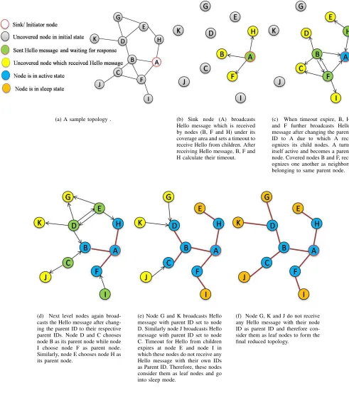
We describe the construction of the reduced topology – formed with the A1 protocol – with the help of an example network shown in figure 1. The topology construction starts in A1 by a node called an initiator node. For protocol im-plementation, we selected a random node as an initiator node and if more than one node initiates the process, the node with the largest ID is chosen. In figure 1(a), the initiator node A

broadcasts a hellomessage to start the topology construction process. The parent node then waits to hear a message with parent ID set to its own ID. We would like to point out that the parent ID field is empty in case of the initiator node.

The nodes B, F and H which are located within the

transmission range ofAreceives thehellomessage (see figure

1(b)). The nodes after the reception of the hello message,

calculates the timeout and enters into sleep mode according to the value of the calculated timeout. As the timeout expires, these nodes discover their neighbors further at different times and sends anotherhellomessage with parent ID field now set

to node A. This allows node A to become an active node.

Nodes B and F are located within each others transmission

range also receives the broadcasted message by both of them. Since in both messages, the parent ID is the same, both nodes recognize them as the children of the same parent node. Similarly, nodeCalso receives the message from nodesBand nodeF. In addition, nodeEand nodeIreceives the message from nodeH and nodeF respectively as shown in figure 1(c).

NodeE and nodeI changes the parent ID field to nodeH

and nodeF respectively and broadcasts the message after the

4

(a) A sample topology . (b) Sink node (A) broadcasts Hello message which is received by nodes (B, F and H) under its coverage area and sets a timeout to receive Hello from children. After receiving Hello message, B, F and H calculate their timeout.

(c) When timeout expire, B, H and F further broadcasts Hello message after changing the parent ID to A due to which A rec-ognizes its child nodes. A turns itself active and becomes a parent node. Covered nodes B and F, rec-ognizes one another as neighbors belonging to same parent node.

(d) Next level nodes again broad-casts the Hello message after chang-ing the parent ID to their respective parent IDs. Node D and C chooses node B as its parent node while node I choose node F as parent node. Similarly, node E chooses node H as its parent node.

(e) Node G and K broadcasts Hello message with parent ID set to node D. Similarly node J broadcasts Hello message with parent ID set to node C. Timeout for Hello from children expires at node E and node I in which these nodes do not receive any Hello message with their own IDs as Parent ID. Therefore, these nodes consider them as leaf nodes and go into sleep mode.

(f) Node G, K and J do not receive any Hello message with their node ID as parent ID and therefore con-sider them as leaf nodes to form the final reduced topology.

Fig. 1. The A1 Protocol

dominators/active nodes. Similarly, node C and D chooses

node B as an active node by sending a message with parent

ID field set to node B. It is worth noting that node C and

node D selected node B as their parent since they received

the message firstly from nodeB due to low value of timeout (see figure 1(d)). This message from node D is also received

at node E which also sent the same message with different

parent ID to nodeD. Since nodeEdo not receive any message with its own parent ID, it discovers itself as a non active node. Similarly, nodeIalso performs in the same manner (see figure 1(e)).

set to nodeDwhich allows nodeDto work as an active node.

On the other hand, node C gets aware due to the message

reception from node J as shown in figure 1(e). In the end,

nodesG,KandI do not receive any message with parent ID set to their own ID and therefore enter into sleep mode after the expiration of calculated timeout. In this manner, a reduced and covered topology is formed in which some nodes work as a virtual backbone for rest of the nodes in the network as shown in figure 1(f).

This completes the description of the A1 protocol. We now provide our experimental setup which is used for the evaluation of the A1 protocol. It is then followed by a detailed discussion on simulation results.

IV. EMPIRICALEVALUATIONFRAMEWORK

This section explains the empirical evaluation framework used for the evaluation of the A1 protocol and other CDS protocols, namely EECDS, CDS Rule K, and A3. We start with the empirical setup that explain the simulation settings and underlying network topologies. In the subsequent section, the topology maintenance techniques are explained. We then provide the definitions of the evaluation metrics on which the protocols are evaluated.

A. Simulation Setup

We evaluated the protocols on a specifically designed simu-lator for WSN topology control protocols [19]. The simusimu-lator –Atarraya– allows the scalability of the underlying network with the ease of selecting different network parameters, such as deployment area, transmission ranges and network size.

For the simulations, we assumed a 600m×600m virtual

space in which nodes are randomly deployed. We have two system parameters, the number of nodes in the space and the common transmission range of nodes. The number of

nodes is increased from 50to250 nodes. We also performed

experiments for the node density beyond250 nodes, however

the trend remains the same for all the four protocols. Similarly,

the maximum transmission range was set to 42min order to

have a connected topology. In addition, nodes sensing range

was set to 10m. In case of indoor topologies, we assumed

a network of 169 nodes for Grid H-V while restricting the

transmission range to 28m. For Grid H-V-D, we increased

the network size to 324 nodes. The network size for indoor

topologies was selected due to the deployment scenario pos-sible as nodes communicate with their horizontal and vertical neighbors in Grid H-V, while in the Grid H-V-D topology, nodes also communicate with their diagonal neighbors.

For the same system parameter settings, we randomly

created 100 connected graph instances and computed a CDS

for each instance for all the four protocols. The initial energy

level of each node was set to 1J with actuation energy

equals 50nJ/bit, while the communication energy was set

to 100P J/bit/m2_{. The nodes communicate with each other}

using full duplex wireless radios. In addition, to use the MAC Protocol Data Unit (MPDU) in the experiments, the message

sizes of all the four protocols were used as explained in earlier section.

B. Topology Maintenance Techniques

Topology maintenance is a process in which a certain desired topological property is maintained to increase the net-work lifetime. Topology maintenance techniques are broadly classified into two categories: static maintenance and dynamic maintenance. In static maintenance, a possible set of disjoint topologies are build at the start of the maintenance operation. The pre-constructed topologies are then rotated based on the time or energy based triggering mechanism. However, static techniques calculate the overhead of pre-constructed topologies at the start, which in most cases, do not represent a realistic scenario as the backbone nodes chosen at the start can behave differently at the later stage. On the other hand, dynamic topology maintenance techniques form a new topology based on the present condition of the network, e.g. as the threshold is reached.

In the next section, we only report the results for dynamic topology maintenance techniques based on energy-threshold. For this purpose, we define the energy threshold to 10% i.e. topology maintenance process is triggered when the network

energy falls by 10%. During topology maintenance, we

as-sumed that a sensed data packet equals 100 bytes for all the four protocols.

C. Definitions of the evaluation metrics

In this section, we now provide formal definitions of the key concepts/metrics used in the evaluation process.

• Message overhead: is defined as the total number of

sent and received packets in the whole network during construction of the topology.

• Energy overhead: is defined as the fraction of the network

energy spent during an experiment.

• Residual energy: is defined as the remaining energy in

the active set of nodes at the end of an experiment.

• Convergence time: is defined as the time taken by a

protocol to construct the topology until the finishing criteria.

• Unconnected nodes: is defined as the number of nodes

which are disconnected from the sink/initiator node at the end of topology maintenance operation.

• Connected sensing area: is defined as the area covered by

the connected nodes at the end of topology maintenance operation.

• Average backbone path length (L): is defined as the

number of edges along the shortest paths for all possible pairs of network nodes. It is given by

L= 1/n(n−1).



X

i,j

d(vi, vj) 

_,

6

50 100 150 200 250

103 104 105 106

Network Size

Total Number of Messages (Log Scale)

EECDS CDS Rule K A3 A1

(a) Message overhead

50 100 150 200 250

10−3 10−2 10−1

Network Size

Energy overhead (log scale)

EECDS CDS Rule K A3 A1

(b) Energy overhead

50 100 150 200 250

0.05 0.1 0.15 0.2 0.25 0.3

Network Size

Residual Energy In CDS

EECDS CDS Rule K A3 A1

(c) Residual energy

Fig. 2. Performance comparison under varying network size.

TABLE I CONVERGENCE TIME(SEC)

Network Size EECDS CDS Rule K A3 A1 50 145.50 89.19 39.34 41.77 100 145.13 102.17 34.31 39.81 150 144.77 114.73 34.04 39.57 200 144.94 127.36 33.90 39.40 250 144.71 140.29 34.21 39.33

Most of the studies in section II consider topology con-struction as the major process thereby ignoring the importance of topology maintenance. Our choice of parameters consid-ers both procedures as integral parts of a topology control protocol. Our choice of message overhead is an extremely important metric as it directly affects the energy consumed in the network. Many authors only consider the number of sent messages as the message overhead. However, we believe that message reception is also critical and, therefore, our definition of message overhead is set accordingly. Similarly, convergence time is also an important measure because new topologies are frequently constructed. If a protocol has higher convergence time, it can affect the overall network performance.

Under topology maintenance, it is important to consider the protocols performance in terms of network connectivity. To analyze this, we selected unconnected nodes parameter to elaborate the performance of the protocols. Finally, covered sensing area at the end of topology maintenance operation is also another important metric. This metric allows us to judge the capability of a protocol in terms of connected nodes covering the area. A protocol is better if it covers more area. Therefore, any protocol designed for WSNs must try to maximize this metric. In the end, an average backbone path length differentiates an easily negotiable network from one which is complicated and inefficient, with a shorter one stated being more desirable in many studies.

V. DISCUSSION ON SIMULATION RESULTS

We have divided the discussion on simulation results into four subsections. We start by discussing the performance of the protocols under varying node densities. We then evaluate all the four protocols in indoor deployment environments:

the Grid H-V and the Grid H-V-D topologies. Subsequently, we discuss the performance of the protocols under dynamic topology maintenance. In the last subsection, we discuss the impact of CDS size on coverage area of WSN’s.

A. Impact of Node Density

The message overhead, energy overhead and residual energy results for varying node densities are shown in figure 2. The number of exchanged messages increases with the increase in the network size. This is due to the reason that increase in the number of nodes also leads to an increase in node degree which also increases the number of exchanged messages. This trend is same for all the four protocols as shown in figure 2(a). However, two phase topology construction leads to high message overhead for EECDS and CDS Rule K protocols. On the other hand, A3 incurs less message overhead due to single phase topology construction. Moreover, it uses less number of messages for topology construction when compared with EECDS and CDS Rule K protocols. In comparison, A1 constructs the topology using one message and has less message overhead than EECDS and CDS Rule K protocols. As can be intuitively argued, an increasing node density leads to higher energy overhead due to an increase in the number of received packets. This trend is visible in figure 2(b) for all the four protocols. However, A1 protocol consumes less energy for the construction of the topology.

Figure 2(c) shows the residual energy among active set of nodes for all the four protocols. Usually, high energy overhead leads to lower residual energy. But, we observed that CDS Rule K ends up with better residual energy resources. This is due to the reason that A3 protocol tries to reduce the virtual backbone by selecting far nodes from the parent node. This results in non-uniform distribution of communication overhead which drains the battery of fewer nodes resulting in lower residual energy levels among nodes in the network. On the other hand, A1 provides better residual energy when compared with all the three protocols. This is because the nodes calculate the timeout with selection criteria which results in balanced virtual backbone.

Grid H−V Grid H−V−D 0

0.5 1 1.5 2 2.5 3x 10

4

Total Number of Messages

CDS Rule K EECDS A3 A1

(a) Message overhead

Grid H−V Grid H−V−D

0 0.2 0.4 0.6 0.8 1 1.2 1.4 1.6x 10

−3

Energy overhead

CDS Rule K EECDS A3 A1

(b) Energy overhead

Grid H−V Grid H−V−D

0 0.1 0.2 0.3 0.4 0.5 0.6 0.7

Residual Energy In CDS

CDS Rule K EECDS A3 A1

(c) Residual energy

Fig. 3. Performance comparison under Grid H-V and Grid H-V-D topologies.

Rule K due to two phase topology construction. On the other hand, A3 and A1 protocol has less convergence time due to a single phase construction of the topology.

B. Indoor Topologies

Figure 3(a) shows the message overhead for all the four protocols under indoor deployment environments. The A1 pro-tocol incurs less message overhead by constructing the topol-ogy with less energy overhead (see figure 3(b)). As the nodes are at equal distances in case of grid environments, nodes only calculate the timeout according to remaining energies of the nodes which results in better residual energy resources for A1 protocol (see figure 3(c)). This is also true for A3 protocol but it fails to perform better due to three way message handshake for the construction of the topology which results in high message and energy overhead. Similarly, Formation of Maximal Independent Set (MIS) and the formation of CDS in EECDS contribute to large number of exchanged messages as the network size is increased. Moreover, CDS Rule K uses a pruning process in which every node updates its two hop neighbors when it is not marked and the process gradually increases as the node density is changed. This results in high energy overhead and less residual energy as shown in figure 3(b) and figure 3(c) respectively.

C. Impact of Topology Maintenance

Figure 4 shows the metric values of all the four protocols under dynamic topology maintenance.

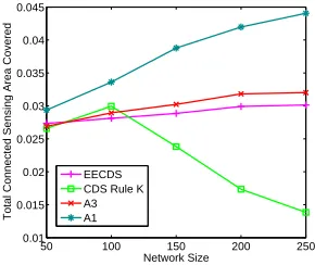
The number of unconnected nodes increases with increase in the network size for all the four protocols. However, CDS Rule K protocol results in large number of unconnected nodes as shown in figure 4(a). In CDS Rule K, nodes remained marked if there is at least one pair of unconnected neighbors. The energy depletion of the marked node leads to higher number of unconnected nodes as compared with the other three protocols. Moreover, it fails to provide better sensing coverage which decreases with the increase in the number of unconnected nodes (figure 4(b)). On the other hand, A3 has less number of unconnected nodes due to its node selection process based on signal strength metric and provides better sensing coverage. In comparison, A1 results in very less number of unconnected

nodes which on the other hand provides better sensing cover-age when compared with all the three protocols.

It is interesting to note that though the number of un-connected nodes increases in EECDS, it results in providing better sensing coverage as shown in figure 4(b). This is due the reason that its two phase topology construction results in forming a proportionate CDS topology with more connected nodes covering the virtual area much better than CDS Rule K protocol.

D. Impact of CDS size on Sensing Coverage

Network’s delivery reliability is a critical parameter that measures the performance of the protocol. We define it as the probability that the sensor nodes can communicate with each other with the increase in the node density. It is given by

R(PS, L) =PSL, (2)

where PS is the probability of success and L is average

backbone path length (virtual backbone) in a CDS. Hence, as L increases, the reliability that a packet will be successfully delivered decreases [20]. However, we noticed that under topology maintenance operation, many nodes get disconnected from the network. Due to this reason, only few nodes remain connected with the sink node at the end of the topology main-tenance (see figure 4(a)). This, on the other hand, computes a smaller average backbone path length. Now, if we model the reliability under fixed probability of success for such a topology, the network reliability appears to be high. On the other side, such a topology fails to provide better coverage.

To elaborate our findings, we generated random topologies of network size varying from 50 to 250 nodes for CDS (CDS RuleK, EECDS and A3) protocols and compared them with the proposed A1 protocol. We computed the average backbone path length for all the four protocols as shown in table II. The results reveals that CDS Rule K protocol provides a very small values for L under varying network size, which on the other hand should provide better reliability

according to equation 2. However, figure 4(b) shows that

8

50 100 150 200 250 50

100 150 200 250

Network Size

Number of Unconnected Nodes

EECDS CDS Rule K A3 A1

(a) Unconnected nodes

50 100 150 200 250 0.01

0.015 0.02 0.025 0.03 0.035 0.04 0.045

Network Size

Total Connected Sensing Area Covered

EECDS CDS Rule K A3 A1

(b) Connected sensing area covered

Fig. 4. Performance comparison under dynamic topology maintenance.

TABLE II

AVERAGE BACKBONE PATH LENGTH(L)

Network Size EECDS CDS Rule K A3 A1 50 3.00 3.00 3.00 3.33 100 3.00 3.33 3.00 3.66 150 3.33 2.66 3.33 4.33 200 3.33 2.00 3.33 4.66 250 3.33 1.66 3.66 5.33

true for EECDS and A3 protocols. On the other hand, L is greater for A1 protocol but it provides better sensing coverage under varying network sizes. Hence, reducing the average backbone path length compromises the coverage region of the protocols. Therefore, size of a CDS should be accounted under topology maintenance while considering coverage area in order to have a better sensing coverage. The A1 protocol forms the reduced topology without any metric desired for the reduction in the size of the CDS. Due to this reason, the number of unconnected nodes as shown in figure 4(a) increases in much slower proportion which on the other hand provides better sensing coverage.

VI. CONCLUSIONS

In this paper, we have investigated the problem of construct-ing a CDS in an energy efficient manner. Our observations reveal that single phase topology construction with fewer number of messages lead towards an efficient protocol. Due to this reason, A1 outperforms other protocols by using far less messages for topology construction. To validate the results, simulations are performed over a large operational spectrum to compare with EECDS, CDS Rule K, and A3 protocols. The results show that A1 has low message complexity and incurs less energy consumption. Moreover, it covers more sensing area under its coverage region and has better connectivity char-acteristics when tested under topology maintenance operation. Therefore, topology maintenance should also be considered for topology construction protocols.

REFERENCES

[1] C. R. Dow, P. J. Lin, S. C. Chen, J. H. Lin, and S. F. Hwang, “A Study of Recent Research Trends and Experimental Guidelines in Mobile Ad Hoc Networks,”Proc. 19th Intl Conf. Advanced Information Networking and Applications (AINA05), pp. 72-77, Mar. 2005.

[2] S. Ni, Y. Tseng, Y. Chen, and J. Sheu, “The Broadcast Storm Problem in a Mobile Ad Hoc Network,” Proc. ACM MobiCom, pp. 152-162, Aug. 1999.

[3] A. Ephremides, J. Wieselthier, and D. Baker, “A Design Concept for Reliable Mobile Radio Networks with Frequency Hopping Signaling,”

Proc. IEEE, vol. 75, no. 1, pp. 56-73, Jan. 1987.

[4] S. Guha and S. Khuller, “Approximation Algorithms for Connected Dominating Sets,”Algorithmica, vol. 20, pp. 374-387, Apr. 1998. [5] K. Mohammed, L. Gewali, and V. Muthukumar, “Generating Quality

Dominating Sets for Sensor Network,”Proc. Sixth Intl Conf. Computa-tional Intelligence and Multimedia Applications (ICCIMA 05), pp. 204-211, Aug. 2005.

[6] D. Kim, Y. Wu, Y. Li, F. Zou, D. Z. Du, “Constructing Minimum Con-nected Dominating Sets with Bounded Diameters in Wireless Networks,”

IEEE Transactions on parallel and distributed computing, Vol. 20, no. 2, Feb. 2009.

[7] R. Ramanathan and R. Rosales-Hain, “Topology control of Multihop Wireless Networks Using Transmit Power adjustment,”IEEE Infocom, pp. 404-413, 2000.

[8] V. Rodoplu and T. H. Meng, “Minimum Energy Mobile Wireless Networks,” IEEE J. Selected Areas in Comm., vol.17, no.8, pp.1333-1344, Aug. 1999.

[9] S. Yang, J. Wu, and F. Dai, Efficient Backbone Construction Methods in MANETs Using Directional Antennas,Proc. 27th Intl Conf. Distributed Computing Systems (ICDCS), 2007.

[10] P. J. Wan, K. M. Alzoubi, and O. Frieder, “Distributed Construction of Connected Dominating Sets in Wireless Ad Hoc Networks,” IEEE INFOCOM, June 2002.

[11] K. M. Alzoubi, P. J. Wan, and O. Frieder, “New Distributed Algorithm for Connected Dominating Set in Wireless Ad Hoc Networks,” Proc. 35th Hawaii Intl Conf. System Sciences (HICSS 02), vol. 9, p. 297, 2002.

[12] K. M. Alzoubi, P. J. Wan, and O. Frieder, “Distributed Heuristics for Connected Dominating Sets in Wireless Ad Hoc Networks,”Journal of Communications and Networks, vol. 4, no. 1, Mar. 2002.

[13] F. Wang, M. T. Thai, and D. Z. Du, “2-Connected Virtual Backbone in Wireless Network,”IEEE Trans. Wireless Comm., 2007.

[14] Y. Wu, F. Wang, M. T. Thai, and Y. Li, “Constructing k-Connected m-Dominating Sets in Wireless Sensor Networks,”Proc. Military Comm. Conf. (MILCOM 07), Oct. 2007.

wireless network interface in an ad hoc networking environment,”Proc. IEEE INFOCOM, vol. 3, pp. 1548-1557, Apr. 2001.

[16] Z. Yuanyuan, X. Jia, and H. Yanxiang, “Energy efficient distributed connected dominating sets construction in wireless sensor networks,” In Proceedings of theACM International Conference on Communications and Mobile Computing, pp. 797-802, 2006.

[17] J. Wu, M. Cardei, F. Dai, and S. Yang, “Extended dominating set and its applications in ad hoc networks using cooperative communication,”

IEEE Trans. on Parallel and Distributed Systems, vol. 17, no. 8, pp. 851-864, 2006.

[18] P. M. Wightman and M. A. Labrador, “A3: A Topology Construction Algorithm for Wireless Sensor Network,” Proc.IEEE Globecom, 2008. [19] P. M. Wightman and M. A. Labrador, “Atarraya: A Simulation Tool to Teach and Research Topology Control Algorithms for Wireless Sensor Networks,” Create-Net 2nd International Conference on Simulation Tools and Techniques, SIMUTools, 2009.

[20] M. Saleem, I. Ullah, S. A. Khayam, and M. Farooq, “On the reliability of Ad hoc routing protocols for loss and delay sensitive applications,”