Multivariable Predictive PID Control
for Quadruple Tank
Qamar Saeed, Vali Uddin and Reza Katebi
Abstract—In this paper multivariable predictive PID controller has been implemented on a multi-inputs multi-outputs control problem i.e., quadruple tank system, in comparison with a simple multi-loop PI controller. One of the salient feature of this system is an adjustable transmission zero which can be adjust to operate in both minimum and non-minimum phase configuration, through the flow distribution to upper and lower tanks in quadruple tank system. Stability and performance analysis has also been carried out for this highly interactive two input two output system, both in minimum and non-minimum phases. Simulations of control system revealed that better performance are obtained in predictive PID design.
Keywords—Proportional-integral-derivative Control, Generalized Predictive Control, Predictive PID Control, Multivariable Systems
I. INTRODUCTION
The three term proportional, integral and derivative (PID) controllers ruled over the process industry for more than six decade, and still existing. The major selling point of PID controllers is due to its simplified structure, robustness and over a wide range of applicability and suitable performance, but limited to simple control problems. In 1939, the first commercial application of PID controller was introduced [1] and a great deal of research and development commenced. Since 1942, numerous PID tuning techniques have been de-veloped and a summary of most popular tuning methods for PID controller are available in [2].
In last few decade, advancement and competition in process industry developed many complex control problems where classical PID were unable to cope and control community strive for better solution. Miller et. al., [3] have illustrated some of the main challenges faced by the control community. Considering the popularity and reliability of PID, many re-searcher tried to develop optimal PID. Rivera et. al., [4] intro-duced an Internal Model Control (IMC) based PID controller design using a first order process model, and this was later extended by Chien [5] for second order process model. Morari and Zafiriou [6], proposed IMC leads to PID controllers for virtually all models common in industrial practice. Wang et. al., [7] proposed a PID controller using a frequency response approach with least squares algorithm to equate with IMC. Rusnak [8] used linear quadratic regulator (LQR) theory to design PID controllers for a fifth order system. Grimble [9], derivedH∞based PID structure. Katebi and Moradi [10] have
Qamar Saeed and Vali Uddin are associated with the Department of Electrical Power and Electronic Engineering, National University of Sciences & Technology Karachi 95350, Pakistan. e-mail: [email protected] and v [email protected]
Reza Katebi is associated with Industrial Control Centre, Uni-versity of Strathclyde, Glasgow, G1 1QE, United Kingdom. e-mail: [email protected]
introduced the predictive PID controller for SlSO systems and Moradi et. al., [11] extended it for MlMO systems in polynomial form. The Generalized Predictive Control (GPC) method proposed by Clarke et. al., [12] is a reasonable rep-resentative of model based predictive control (MPC) methods and one of the most general way of posing the process control problem in time domain [13]. Tan et. al., [14] have presented a PID control design based on the GPC approach for a second order system with time delay but limited to single-input single output (SISO) systems. In this paper, we have develop a multi-input multi-output Predictive PID controller using the same approach as used by Tan et. al., [15] for his SISO systems.
In the recent past, multi-variable control system design have been in great demand and need much attention in the process industry and academia. In many processes, when some or all of the manipulated variable affects more than its corresponding controlled variable, mean there are some interaction between the controlled variable, which may result in poor performance or even in instability of control process. When the interaction are not negligible, the plant must be considered as multiple inputs and multiple outputs. In this paper, a highly interactive multi-variable process has been considered i.e., quadruple tank problem. This multi-variable systems contains a transmission zeros, which can vary from left half plane (minimum phase) to right half plane (non-minimum phase) depending on the ratio of the flow to upper and lower tanks [16].
The paper has been organized as follows: Section II briefly describe the model development of real processes. Manual multi-loop PI and predictive PID control design techniques has been discussed in section III and IV respectively. Stability analysis has been conducted in Section V. Performance anal-ysis and simulation results are available in section VI. Finally, the conclusions are given in section VII.
II. MODELDEVELOPMENT
Johansson [16] described a laboratory quadruple-tank pro-cess which consists of four interconnected water tanks and two pumps as shown in fig. 1. The first principle mathematical model for this process using mass balances and Bernoulli’s law is
dh1
dt = −
a1 A1
2gh1+Aa3 1
2gh3+ γA1k1 1 v1 dh2
dt = −Aa22
2gh2+Aa4 2
2gh4+ γA2k2 2 v2 dh3
dt = −
a3 A3
2gh3+(1−Aγ2)k2
3 v2
dh4
dt = −
a4 A4
2gh4+(1−Aγ1)k1
Fig. 1. Schematic diagram for Quadruple Tank process
whereγi is the flow distribution to lower and diagonal upper
tank,Ai is the cross-section area,ai is the outlet hole
cross-section andhi is the water level, in tank irespectively.
There are two inputs (manipulators) and two outputs (con-trolled variable) in quadruple tank system, and control ob-jective is to maintain water level in lower tanks around its setpoint with the manipulation of water flow with two pumps. The process inputs arev1andv2and the outputs arey1=kch1 andy2=kch2.
The voltage applied to Pumpiisvi and the corresponding
flow iskivi. The parametersγ1, γ2∈(0,1)are valves setting for the distribution of flow to lower and upper diagonal tank respectively. The flow to Tank 1 is γ1k1v1 and the flow to Tank4is (1−γ1)k1v1 and similarly for Tank 2 and Tank3 as shown in fig. 1. Thegis denoted as acceleration of gravity. The parameter values of the laboratory process and operating parameter for minimum (P−) and non-minimum phases (P+) are given in [16], also shown in table 1 and table 2 respectively. This typical system has two finite zeros forγ1, γ2∈(0,1). One always lie in the left half-plane, but the other can be placed either in the left or the right half-plane depending on the valve setting ofγ1, γ2.
If1 < γ1+γ2 ≤ 2 then system is minimum phase, means transmission zero is in left half plane.
If0≤γ1+γ2<1then system is non-minimum phase, means transmission zero is in right half plane.
Ifγ1+γ2 = 1 then system has transmission zero at origin, a difficult case to handle using simple multi-loop PID control system design without de-coupler.
Parameters Units Values A1,A3 [cm2] 28
A2,A4 [cm2] 32
a1,a3 [cm2] 0.071
a2,a4 [cm2] 0.057
kc [V/cm] 0.5 g [cm/s2] 981
TABLE I
PARAMETER VALUE FORQUADRUPLETANK
The linearized state-space equation at operating points xi = hi − h0i and ui = vi − vi0 is given
Operating Values Units P− P+
(h01,h02) [cm] (12.4,12.7) (12.6,13.0)
(h03,h04) [cm] (1.8.1.4) (4.8,4.9)
(v0
1,v20) [V] (3.00,3.00) (3.15,3.15)
(k1,k2) [cm2/V s] (3.33,3.35) (3.14,3.29)
(γ1,γ2) - (0.70,0.60) (0.43,0.34) TABLE II
OPERATING PARAMETER FOR MINIMUM(P−)AND NON-MINIMUM(P+)
PHASES
in [16]
dx
dt =
⎛ ⎜ ⎜ ⎝
−1
T1 0
A3 A1T3 0
0 −1
T2 0
A4 A2T4
0 0 −1
T3 0
0 0 0 −1
T4
⎞ ⎟ ⎟ ⎠x
+
⎛ ⎜ ⎜ ⎜ ⎝
γ1k1
A1 0
0 γ2k2
A2 0 (1−γ2)k2
A3 (1−γ1)k1
A4 0
⎞ ⎟ ⎟ ⎟ ⎠u
y = k0c k0 0 0
c 0 0
x (2)
where the time constants areTi= Aaii
2h0
i
g .
Linearized transfer function matrix model for both mini-mum (P−) and non-minimum (P+) phases are given in [16] and [17].
III. MANUAL MULTI-LOOPPI CONTROL
The discrete position and velocity form of PID controller are described by equations (3) and (4) respectively [10].
u(k) =kpe(k) +ki k
j=1
e(j) +kd[e(k)−e(k−1)] (3)
Δu(k) =u(k)−u(k−1) =kp[e(k)−e(k−1)] + +kie(k) +kd[e(k)−2e(k−1) +e(k−2)](4)
where,kp,ki andkdare the proportional, integral and
deriva-tive gains, respecderiva-tively.
Johansson [16] applied multi-loop PI controller on quadru-ple tank manually for both minimum and non-minimum phase configuration in frequency domain. However, in this section same tuning parameters are implemented in control system design using state space formulation. All simulation results have been discussed in section VI in comparison with [16].
IV. PREDICTIVEPID CONTROL
Consider a two-input two-output square multi-variable sys-tem is given as
y1 y2
= gg11 g12 21 g22
u1 u2
(5)
In equation (5), eachgij (where i, j = 1,2) contains a
sub-system which can be represented as [14] and [15]
gij(s) = (s+dsa)(+sc+b)e−sL (6)
The equation (6) in discrete-time transfer function can be represented as
´
gij(z) = ´
b1z+ ´b2
z2+ ´a1z+ ´a2z−td (7) With some algebraic manipulation in equations (5 - 7), two multi-input single output (MISO) model can be obtained as,
z2+ ´a1
11z+ ´a211 0 0 z2+ ´a1
22z+ ´a222
y1(t) y2(t)
= ´b011z+ ´b111 ´b012z+ ´b112 ´b0
21z+ ´b121 ´b022z+ ´b122
u1(t) u2(t)
(8)
The error to the controller is represented ase=yd−y, where ydis the setpoint andyis the controlled output, then in terms
of error, withyd= 0, equivalent equation can be represented
as,
e1(k+ 1) = ´a111e1(k)−´a211e(k−1) −´b0
11u˜1(k)−´b012u˜2(k) (9) e2(k+ 1) = ´a122e2(k)−´a222e(k−1)
−´b0
21u˜1(k)−´b022u˜2(k) (10) where
˜
u1(k) = u1(k) + ´b1
11 ´b0
11
u1(k−1)
˜
u2(k) = u2(k) + ´b1
12 ´b0
12
u2(k−1)
Equations (9 - 10) can be represented in state space form as X(k+ 1) =AX(k) +Bu˜(k) (11) where A= ⎛ ⎜ ⎜ ⎜ ⎜ ⎜ ⎜ ⎝
0 1 0
−´a2
11 −a´111 0
0 1 1
0 1 0
−´a2
22 −a´122 0
0 1 1
⎞ ⎟ ⎟ ⎟ ⎟ ⎟ ⎟ ⎠
,B= ⎛ ⎜ ⎜ ⎜ ⎜ ⎜ ⎜ ⎝ 0 0
−´b0
11 −´b012
0 0
0 0
−´b0
21 −´b022
0 0 ⎞ ⎟ ⎟ ⎟ ⎟ ⎟ ⎟ ⎠
X(k) =
⎛ ⎜ ⎜ ⎜ ⎜ ⎜ ⎜ ⎝
e1(k−1) e1(k) θ1(k) e2(k−1)
e2(k) θ2(k)
⎞ ⎟ ⎟ ⎟ ⎟ ⎟ ⎟ ⎠
,u˜(k) = ⎛ ⎜ ⎜ ⎝
˜
u11(k) ˜
u12(k) ˜
u21(k) ˜
u22(k) ⎞ ⎟ ⎟ ⎠
andθi=kj=1ei(j)is the integral error.
Usingp and m prediction and control horizons respectively,
the predicted error in compact form can be represented as [14] and [15],
¯
X=¯LAX(k) +BMU˜ (12) where
¯
X = XT(k+ 1) XT(k+ 2) · · · XT(k+p) T
¯L = ⎛ ⎜ ⎜ ⎜ ⎝ I A .. . Ap−1
⎞ ⎟ ⎟ ⎟ ⎠
BM = ⎛ ⎜ ⎜ ⎜ ⎜ ⎝
B 0 · · · 0
AB B · · · ... ..
. ... . .. 0 Ap−1B Ap−2B · · · Ap−mB
⎞ ⎟ ⎟ ⎟ ⎟ ⎠ ˜
U = ˜u(k) ˜u(k+ 1) · · · u˜(k+m−1) T
Since GPC is an optimal control strategy, therefore a perfor-mance index or cost function must be minimized in order to obtain an optimal control signal. Considering the following cost function
J= p
l=1
x(k+l)2 Q(l)+
m
j=1
u(k+j−1)2
R(j) (13)
where Q andR are the error and control weighting matrices respectively. Substitution of prediction equation (12) in cost function (13) i.e., an optimization step, resulted an optimal control sequence, like [14] and [15]
¯
U=−[BT
MQBM+R]−1[BTMQLA]X(k) (14)
Under the receding horizon principle, only the first value of the optimal control sequence is applied at each sampling time while the rest are discarded. Therefore,
˜
u(k−td) = −H[BTMQBM+R]−1[BMTQLA]X(k),
= −DX(k) (15)
where D=H[BTMQBM+R]−1[BMTQLA]
andH= I 0 . . . 0
From equation (15), it follows that u˜ = −DX(k + td),
which means that current control value depends on the future predicted state. In case of significant time delay, this problem would be solved in two different range i.e., 0≤ k < td and k≥td, [14] and [15]. However, in absence of time delay (i.e., td= 0) then control law would simply be
˜
u=−DX(k) (16)
Similarly, ⎛ ⎜ ⎜ ⎝ ˜
u11,k ˜
u12,k ˜
u21,k ˜
u22,k
⎞ ⎟ ⎟ ⎠= ⎛ ⎜ ⎜ ⎝
D11 0
D12 0
0 D21 0 D22
⎞ ⎟ ⎟ ⎠ XX12
(17)
There is no significant time delay in quadruple tank system, so PID tuning parameters would only be consider for k≥td
⎧ ⎨ ⎩
KP =−(K1(td) +K2(td)) KI =−K3(td)
KD =K1(td)
⎫ ⎬
Earlier we have assumed that,
˜
u11,k = u1,k+ ´b1
11 ´b0
11
u1,k−1 (18)
˜
u12,k = u2,k+ ´b1
12 ´b0
12
u2,k−1 (19)
˜
u21,k = u1,k+ ´b1
21 ´b0
21
u1,k−1 (20)
˜
u22(k = u2,k+ ´b1
22 ´b0
22
u2,k−1 (21)
On combining equations (18 & 20) and (19 & 21), we obtain
˜
u11,k+ ˜u21,k = 2u1,k+ ( ´b1
11 ´b0
11 +´b121
´
b0 21
)u1,k−1 (22)
˜
u12,k+ ˜u22(k = 2u2,k+ ( ´b1
12 ´b0
12 +´b122
´
b0 22
)u2,k−1 (23)
Similarly,
u1,k = 12
(˜u11,k+ ˜u21,k)−( ´b1
11 ´b0
11 +´b121
´b0 21
)u1,k−1
(24)
u2,k = 12
(˜u12,k+ ˜u22(k)−( ´b1
12 ´b0
12 +´b122
´b0 22
)u2,k−1
(25)
V. STABILITYANALYSIS
The stability is one of the major concern in all control system design. In case of linearized model, the stability of overall closed loop system is determined by characteristic equation.
In terms of transfer function two input two output (TITO) system can be described as,
y1 = g11u1+g12u2 (26)
y2 = g21u1+g22u2 (27)
In multi-loop PI control tuning for minimum phase problem, the control law is
u1 = gc1(yd,1−y1) (28) u2 = gc2(yd,2−y2) (29) As setpoint do not play any role in system stability, so let yd,2= 0. Now substituting the equation (29) in equation (26) with algebraic manipulation, we get the characteristic equation for minimum phase (C.Emp) as,
C.Emp= 1+gc1g11+gc2g22+gc1gc2(g11g22−g12g21) (30) Similarly, the control law for non-minimum phase multi-loop PID controllers are described as
u1 = gc1(ysp,2−y2) (31) u2 = gc2(ysp,1−y1) (32) On substitution of equations (31-32) in equations (26-27) yield
1 +g12gc1 g11gc2 g22gc1 1 +g21gc2
y1 y2
=
g12gc1 g11gc2 g22gc1 g21gc2
ysp,1 ysp,2
(33)
Eventually, characteristic equation for non-minimum phase (C.Enmp) obtained as
C.Enmp= (1 +g12gc1)(1 +g21gc2)−gc1gc2g11g22 (34) Johansson [16] describe that non-minimum phase configura-tion in quadruple tank system, is relatively a difficult control problem as one of the pole is very close to unit circle.
The stability of Predictive PID design based on GPC can also be carried out in a similar manner. From (24-25), we can obtainedu1,k andu2,k as
u1,k =
2 + ´b111 ´
b0 11
+´b121 ´
b0 21
z−1−1(˜u
11,k+ ˜u21,k)(35)
u2,k =
2 + ´b112 ´
b0 12
+´b122 ´
b0 22
z−1−1(˜u
12,k+ ˜u22,k)(36)
From equation (17), we have,
˜
u11,k+ ˜u21,k = D11 D21 X(k) (37) ˜
u12,k+ ˜u22,k = D12 D22 X(k) (38) where X(k)is defined as,
X(k) = X1(k) X2(k) T (39)
in which
X1(k) = e1(k−1) e1(k−1) θ1(k) T X2(k) = e2(k−1) e2(k−1) θ2(k) T Using equations (26 - 27) and (35 - 38), a characteristic equa-tion can be obtained and stability of the closed loop system are determined. In predictive PID design, we obtained the PID tuning parameters on the basis of GPC tuning parameters and equate to the PID tuning parameters in result as mentioned in section IV. Moreover, all simulation results revealed that systems are stable along the selected tuning parameters.
VI. PERFORMANCEANALYSIS& SIMULATIONRESULTS
The multi-loop PI tuning parameters are obtained from [16], where (K1, Ti1) = (3.0,30) and (K2, Ti2) = (2.7,40) for minimum phase (P−) while (K1, Ti1) = (1.5,110) and (K2, Ti2) = (−0.12,220) for non-minimum phase (P+) system respectively. In this paper, simulation have been carried out in time domain using state space approach in compari-son with earlier Johanscompari-son [16], frequency domain approach. Moreover, we have also plotted the upper tanks (i.e., tank 3 and tank 4) level along with the lower tanks (i.e., tank 1 and tank 2), for better illustration and understanding.
For minimum phase, we have observed a peak (i.e., overshoot) upto 7.45 with settling time is 60 sec as shown in fig. 2, while [16] indicated peak upto 7.3 with settling time 80 sec.
0 100 200 300 1
1.5 2
h3
0 100 200 300
1 1.5 2
h4
0 100 200 300
6 7 8
y1
=k
c
h1
0 100 200 300
6 6.5 7
y2
=k
c
h2
0 100 200 300
0 5 10
time u1
0 100 200 300
2 4 6 8
[image:5.595.60.295.116.381.2]time u2
Fig. 2. Manual PID design for minimum phase
0 100 200 300
1 1.5 2 2.5
h3
0 100 200 300
1 1.5 2 2.5
h4
0 100 200 300
6 6.5 7 7.5
y1
=k
c
h1
0 100 200 300
6 6.5 7 7.5
y1
=k
c
h2
0 100 200 300
2 3 4 5
time u1
0 100 200 300
2 3 4 5
[image:5.595.311.549.120.379.2]time u2
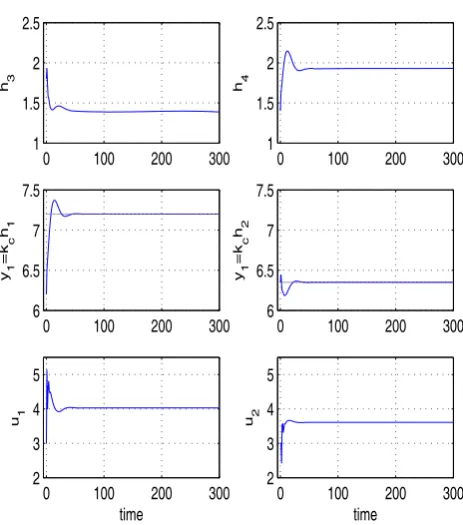
Fig. 3. Predictive PID design for minimum phase
0 1000 2000 3000 4000
0 5 10 15
h3
0 1000 2000 3000 4000
0 5 10 15
h4
0 1000 2000 3000 4000
4 6 8
y1
=k
c
h1
0 1000 2000 3000 4000
4 6 8 10 12
y2
=k
c
h2
0 1000 2000 3000 4000
0 2 4 6 8
time u1
0 1000 2000 3000 4000
0 2 4 6 8
[image:5.595.61.293.456.719.2]time u2
Fig. 4. Manual PID design for non-minimum phase
0 500 1000 1500
4 6 8 10
h3
0 500 1000 1500
2 4 6
h4
0 500 1000 1500
5 6 7 8
y1
=k
c
h1
0 500 1000 1500
5 6 7 8
y2
=k
c
h2
0 500 1000 1500
3 4 5
time u1
0 500 1000 1500
3 4 5
time u2
[image:5.595.314.550.461.720.2]fig. 4, while [16] indicated no inverse response and overshoot only upto7.9with settling time around 1200 sec (i.e., 15 times more than minimum phase).
Our simulation results are based on state space model in comparison with [16], which are based on transfer function model, the results we have obtained are slightly different than [16], but the trends are almost the same. Moreover, we are in concordance that non-minimum phase problem is much more difficult to tackle using manual multi-loop PID control design as concluded in [16].
In section IV, we have developed a MIMO predictive PID controller for quadruple tank problem using the same technique as given in [14] and [15] for SISO system. For minimum phase, we have used prediction horizon asN1= 1, N2 = 40 and control horizon as Nu = 40 with weighting R= ρI2 = 10I2 and Q = I3 and observed the closed loop response ofy1with peak as7.35for setpointysp,1= 7.2while y2regain its initial position within settling time i.e., 35 sec as shown in fig. 3.
Similarly for non-minimum phase, we have used the predic-tion horizonN1= 1,N2= 100 and control horizonNu= 2
with weighting Q = I3 and R = ρI2 = 1000I2 an inverse response have been observed with settling time around 700 sec i.e., more than 20 times of the minimum phase problem as shown in fig 5. However, in real plant i.e., a nonlinear system result could be slightly different as the water drain from any respective tank depends on the square root of its level, not directly to its level.
VII. CONCLUSIONS
The structure of the P-PID is not much different from the conventional PID, therefore implementation does not make any difference. The effectiveness of all these methods have been well illustrated in simulations.
It has been observed that in each design technique, non-minimum phase is quite difficult to control. Multivariable system with unstable transmission zeros usually come across with internal instability problems i.e., a difficult aspect to control a process with RHPT zero canceled by a RHP pole. An important characteristic of RHPT zeros of input multi-output (MIMO) systems is that it contains hidden dynamics.
ACKNOWLEDGMENT
This research work is financially supported by Higher Edu-cation Commission of Pakistan and Industrial Control Centre, University of Strathclyde, UK.
REFERENCES
[1] Kristiansson, B. and B. Lennartson, Robust Tuning of PI and PID Con-trollers - Using Derivative Action Despite Sensor Noise,IEEE Control System Magazine, 26(1), (2006), 55–68
[2] Cominos, P., and N. Munro, PID Controllers: recent tuning meth-ods and design to specification, IEEE Control System Maga-zine, 149(1), (2002), 46–53.
[3] Miller. R.M., S.L. Shah, R.K. Wood and E.K. Kwok, Predictive PID,ISA Transaction, (1999), 38, 11–23.
[4] Rivera, D.E., S. Skogestad and M. Morari, Internal Model Control 4. PID Controller Design. Ind. Eng Chem. Proc. Design and Develop-ment, 25, (1986), 252–265.
[5] Chein, I.L., IMC-PID Controller Design-An Extension,IFAC Proceeding Series, 6, (1988), 147–152.
[6] Morari, M. and E. Zafiriou, Robust Process Control, Printice Hall, (1989). [7] Wang, Q.G., C.C. Hang and X.P. Yang, Single Loop Controller Design Via IMC Principles, InProceeding Asian Control Conference, Shanghai, P.R.China, (2000).
[8] Rusnak, I., Generalized PID Controllers,Proc. 7th IEEE Medit. Confer-ence on Control & Automation, MED 99, Haifa, Israel, (1999). [9] Grimble, M.J., H-infinity PID Controllers, Trans. IMC,
13(5), (1991), 112–120.
[10] Katebi, M.R. and M.H. Moradi, Predictive PID Controllers,IEE Proc. Control Theory Application, 148(6), (2001), 478–487.
[11] Moradi. M.H., M.R. Katebi, and M.A. Johnson, The MIMO Predictive PID Controller Design,Asian Journal of Control, 4(4), (2002), 452–463. [12] Clarke. D.W., C. Mohtadi and P.S. Tuffs, Generalized Predictive
Control-Part I. The Basic Algorithm,Automatica, 23(2), (1987), 137–148. [13] Bordons, C., and Camacho, E.F., A Generalized Predictive Controller
for a Wide Class of Industrial Processes,IEEE Transactions on Control Systems Technology, 6(3), (1998), 372–387.
[14] Tan, K.K., S.N. Huang, and T.H. Lee, Development of a GPC-based PID Controller for Unstable System with Dead Times,ISA Transaction , 39, (2000), 57–70.
[15] Tan, K.K., T.H. Lee, S.N. Huang, and F.M. Leu, PID Controller Design Based on a GPC Approach,Ind. Eng. Chem. Res., 41, (2002), 2013–2022. [16] K. H. Johansson, The Quadruple-Tank Process: A Multivariable Labo-ratory Process with an Adjustable Zero, IEEE Transactions on Control Syatems Technology, 8(3), (2000), 456–465.