A numerical study of 2D integrated RBFNs incorporating Cartesian grids for solving 2D elliptic differential problems

A numerical study of 2D integrated RBFNs

incorporating Cartesian grids for solving 2D elliptic

differential problems

N. Mai-Duy

and T. Tran-Cong

Computational Engineering and Science Research Centre

Faculty of Engineering and Surveying,

The University of Southern Queensland, Toowoomba, QLD 4350, Australia

Submitted to

Numerical Methods for Partial Differential Equations

,

15-Dec-2008; revised, 25-May-2009

Short title: 2D-IRBFN Cartesian-grid technique

AbstractThis paper reports a numerical discretisation scheme, based on two-dimensional integrated radial-basis-function networks (2D-IRBFNs) and rectangular grids, for solving

second-order elliptic partial differential equations defined on 2D non-rectangular domains.

Unlike finite-difference and 1D-IRBFN Cartesian-grid techniques, the present

discretisa-tion method is based on an approximadiscretisa-tion scheme that allows the field variable and

its derivatives to be evaluated anywhere within the domain and on the boundaries,

re-gardless of the shape of the problem domain. We discuss the following two particular

strengths, which the proposed Cartesian-grid-based procedure possesses, namely (i) the

implementation of Neumann boundary conditions on irregular boundaries and (ii) the

use of high-order integration schemes to evaluate flux integrals arising from a

control-volume discretisation on irregular domains. A new preconditioning scheme is suggested

to improve the 2D-IRBFN matrix condition number. Good accuracy and high-order

con-vergence solutions are obtained.

Keywords: integrated radial basis function network; Cartesian grid; irregular domain;

Neumann boundary condition; control-volume discretisation; point-collocation

discretisa-tion

1

INTRODUCTION

Discretisation techniques require the replacement of the domain of interest with a union

of small elements, a collection of control volumes, a Cartesian grid or a set of discrete

points. Generating a Cartesian grid or a set of discrete points is seen to be much more

economical than generating a finite-element mesh, particularly for the case of

irregularly-shaped domains. As a result, considerable effort has been put into the development of

Cartesian-grid-based techniques and meshless techniques.

Cartesian-grid techniques, difficulties lie in the handling of irregular boundary geometries.

Since the irregular boundary does not generally pass through grid nodes (regular points),

one expects to have a change in grid spacing in all directions for interior points adjacent

to the boundary. It has been shown that a rapid change of the grid size can result in a

substantial deterioration in accuracy (e.g. [1]). A variety of techniques have been explored

to overcome this problem. Examples include higher-order boundary fitting schemes, where

error bounds for the quadratic boundary treatment are derived, (e.g. [2,3]) and embedded

boundary techniques (e.g. [4,5]). There are further complications for the case of Neumann

boundary conditions. Expressions for computing a gradient boundary condition embrace

first-order derivatives in both coordinate directions. However, at an irregular boundary

point, one is given explicitly information about the change of the field variable in one

coordinate direction only. Special treatments are required. Typically, supplementary

approximations are introduced at the boundary (e.g. [6-8]) or rectangular grids are formed

in a way that boundary points are also grid nodes (e.g. [9]). If one uses a control-volume

approach (subregion collocation) for the discretisation, the accuracy of the technique

depends on both the approximation of gradients (e.g. diffusive fluxes) and the evaluation

of integrals involving these gradients. For the latter, assume that the flux evaluations are

sufficiently accurate, the midpoint rule is capable of yielding second-order accuracy only

as discussed in [10].

Radial-basis-function networks (RBFNs) are known as a powerful tool for the

approxima-tion of scattered data. Their applicaapproxima-tion to the soluapproxima-tion of partial differential equaapproxima-tions

(PDEs) has received a great deal of attention over the last 15 years (e.g. [11] and

ref-erences therein). It is easy to implement RBF collocation methods and they can give a

high-order convergence solution. On the other hand, the RBF matrices are fully

popu-lated and their condition numbers grow quickly with increasing number of RBF centres.

A number of approaches, such as local approximations (e.g. [12,13]), domain

(e.g. [18,19]), have been presented, towards the solution of large-scale problems.

Integrated RBFNs (IRBFNs) have some advantages over differentiated RBFNs (DRBFNs)

in certain types of problems such as those involving the approximation of high-order

derivatives, the implementation of multiple boundary conditions, and the enforcement

of second-order continuity of the approximate solution across the subdomain interfaces

(e.g. [20-22]). In the context of Cartesian-grid techniques, IRBFNs were employed to

represent the field variable on each grid line (1D-IRBFNs), which allows a larger number

of nodes to be employed (e.g. [23-25]). Because 1D-IRBFN approximation schemes with

respect to the two coordinate directions are independent, difficulty is encountered for

irregular domains when one tries to implement normal derivative boundary conditions

and use Gaussian quadrature to evaluate flux integrals. In [24], a technique for generating

a non-uniform grid where the boundary points coincide with regular mesh points [9]

was adopted to implement Neumann boundary conditions. In this paper, we discuss

the use of 2D-IRBFNs over the whole domain that has the ability to overcome these

difficulties. Furthermore, a new preconditioning scheme and a hybrid numerical procedure

are proposed to enhance the performance of the present Cartesian-grid-based technique.

The remainder of the paper is organised as follows. In Section 2, a brief review of

in-tegrated RBFNs is given. In Section 3, the proposed Cartesian-grid-based technique

incorporating 2D-IRBFNs is described and its performance is investigated numerically.

Emphasis is placed on the discussion about some strengths and weaknesses of 2D-IRBFNs

2

TWO-DIMENSIONAL INTEGRATED RBFNs ON

CARTESIAN GRIDS

In the remainder of the paper, we will use

• the notation b[] for a vector/matrix [] that is associated with 1D-IRBFNs, a grid line or a segment of the boundary,

• the notation e[] for a vector/matrix [] that is associated with 2D-IRBFNs or the whole set of grid lines,

• the notation [](η) to denote selected rows η of the vector [],

• the notation [](η,θ) to denote selected rows η and columns θ of the matrix [],

• the notation [](:,θ) to denote all rows of the matrix [],

• the notation [](η,:) to denote all columns of the matrix [], and

• the notation cond([]) to denote the the 2-norm condition number of the matrix [].

The domain of interest, which can be rectangular or non-rectangular, is embedded in a

Cartesian grid of density N1 ×N2. In the case of non-rectangular domains, grid nodes

outside the domain are removed. Boundary points are generated through the

intersec-tion of the grid lines and the boundaries of the domain. The construcintersec-tion of the RBF

approximations can be based on differentiation or integration. For the latter, which is

employed in this study, the highest-order derivatives of the field variable in a given PDE

are decomposed into RBFs. Approximate expressions for lower-order derivatives and the

field variable itself are then obtained through integration. For the solution of second-order

PDEs on 2D domains, the integral scheme will start with

∂2_u(x)

∂x2 =

N

X

where u is the field variable, x the position vector,xj the j-component of x(j = [1,2]),

N the number of RBF centres (interior and boundary points) associated with the xj grid lines (N =N1N2 for a rectangular domain), w the network weight and G(x) the RBF.

Integrating (1) with respect to xj leads to

∂u(x)

∂xj =

N

X

i=1

w(i)H(i)(x) +C1(xk), (2)

u(x) = N

X

i=1

w(i)H(i)(x) +xjC1(xk) +C2(xk), (3)

where H =R Gdxj, H =

R

Hdxj, and C1 and C2 are the constants of integration which

are univariate functions of the variable other than xj (i.e. xk (k 6=j)). For points lying on a grid line that is parallel to the xj direction, expressions (2) and (3) will have the same values of C1 and C2.

We also employ IRBFNs to represent the variation of the constants of integration. These

approximate functions are expressed in terms of the nodal values of C1 and C2 (the

physical space) rather than in terms of the RBF weights/coefficients used in past work

(e.g. [26]).

The construction process for C1(xk) is exactly the same as that for C2(xk). To simplify

the notation, some subscripts are dropped. The functionC(xk) is constructed through

d2_C(xk)

dx2 k = Nk X i=1

w(i)g(i)(xk), (4)

dC(xk)

dxk =

Nk

X

i=1

w(i)_h(i)_{(xk) +c}

1, (5)

C(xk) = Nk

X

i=1

w(i)¯h(i)(xk) +xkc1+c2, (6)

wherec1 and c2 are the constants of integration which are simply unknown numbers, and

Collocating (6) at the local grid pointsx(_ki) with i={1,2,· · · , Nk}leads to

b

C =Tb

      b w c1 c2     

, (7)

where Cb and w_b are the vectors of length Nk, andTb the transformation matrix of dimen-sions Nk×(Nk+ 2)

b

C =C(x(1)_k ), C(x_k(2)),· · · , C(x_k(Nk))T = C(1), C(2),· · ·, C(Nk)T _,

b

w= w(1), w(2),· · ·, w(Nk)T _,

b T =          ¯

h(1)(x(1)k ), h¯(2)(x

(1)

k ), · · · , ¯h(Nk)(x

(1)

k ), x

(1)

k , 1 ¯

h(1)_(x(2)

k ), h¯(2)(x

(2)

k ), · · · , ¯h(Nk)(x

(2)

k ), x

(2)

k , 1

... ... . .. ... ... ...

¯

h(1)_(x(Nk)

k ), ¯h(2)(x

(Nk)

k ), · · · , ¯h(

Nk)(x(Nk) k ), x

(Nk)

k , 1

         .

Taking (7) into account, the value of (6) at an arbitrary point xk can be computed in terms of nodal values ofC as

C(xk) = ¯h(1)(xk),¯h(2)(xk),· · ·,¯h(Nk)_{(xk), x}

k,1 bT+C,b (8) or

C(xk) = Nk

X

i=1

P(i)_(xk)C(i)_{, (9)}

where P(i)_{(xk) is the product of the first vector on RHS of (8) and the ith column of}

b

T+_{, and T}b+ _{the generalised inverse of T}b _{of dimensions (N}

Substitution of (9) into (2) and (3) yields

∂u(x)

∂xj =

N

X

i=1

w(i)_H(i)_{(x) +}

Nk

X

i=1

P(i)_(xk)C(i)

1 , (10)

u(x) = N

X

i=1

w(i)H(i)(x) + Nk

X

i=1

xjP(i)(xk)C₁(i)+ Nk

X

i=1

P(i)(xk)C₂(i). (11)

For convenience of presentation, expressions (1), (10) and (11) can be rewritten as

∂2_u(x)

∂x2

j =

N_X+2Nk i=1

w(i)G(i)(x), (12)

∂u(x)

∂xj =

N_X+2Nk i=1

w(i)_H(i)_{(x), (13)}

u(x) =

NX+2Nk i=1

w(i)_H(i)_{(x), (14)}

where

{G(i)(x)}N+2Nk

i=N+1 ≡ {0} 2Nk i=1,

{H(i)(x)}N+Nk

i=N+1 ≡ {P(

i)_(xk)}Nk i=1,

{H(i)(x)}N+2Nk

i=N+Nk+1 ≡ {0} Nk i=1,

{H(i)(x)}N+Nk

i=N+1 ≡ {xjP(i)(xk)}Ni=1k,

{H(i)(x)}N+2Nk

i=N+Nk+1 ≡ {P

(i)_(xk)}Nk i=1,

{w(i)}N+Nk

i=N+1 ≡ {C (i)

1 }

Nk i=1, and

{w(i)_}N+2Nk

i=N+Nk+1 ≡ {C

(i)

2 }

Nk i=1.

We seek an approximate solution in terms of nodal values of the field variable. To do

Collocating (14) at the nodal points associated with the xj grid lines,

x(i) N_i=1, leads to

e T       e w b C1 b C2     

=u,e (15)

whereTe is aN×(N+2Nk) matrix,w_e= w(1)_{, w}(2)_{,· · · , w}(N)T_,Cb

1 =

C₁(1), C₁(2),· · · , C₁(Nk)T,

b

C2 =

C₂(1), C₂(2),· · · , C₂(Nk)T, and _eu= u(x(1)), u(x(2)),· · · , u(x(N))T. The transforma-tion matrix Te has the entriesTeli =H

(i)

(x(l)) for 1≤l≤N and 1≤i≤(N + 2Nk). It is noted that at a grid nodeP(i)_(x(j)

k ) is equal to 0 if i6=j and 1 if i=j. Solving (15) for the coefficient vector yields

      e w b C1 b C2      = e

T+u,_e (16)

where Te+ _{is the generalised inverse ofT}e_.

The values of first- and second-order derivatives of u at the nodal points associated with the xj grid lines can then be computed in terms of nodal variable values as

g∂u ∂xj

=HeTe+_{u,e (17)}

g

∂2_u

∂x2

j

=GeTe+_{eu, (18)}

Expressions (17) and (18) can be rewritten in compact form

g∂u ∂xj

=De′

ju,e (19)

g

∂2_u

∂x2

j

=De′′

jeu, (20)

where De′

j = HeTe+ and De

′′

j =GeTe+ are the first and second-order differentiation matrices in the physical space.

Consider a Poisson equation ∇2_{u = b with Dirichlet boundary conditions. Using point}

collocation, it can be transformed into

e

Au_e(θ)=

e

D′′₁₍η,θ)+De

′′

2(η,θ)

e

u(θ) =eb(η), (21)

where Ae is the system matrix, and η and θ the two sets of indices representing the interior points. It is noted that η and θ are identical and the nomenclature was given at the beginning of this section. The integral solution procedure involves computing the

transformation matrix Te and the system matrixAe. From a computational point of view, it is desirable to haveTe and Aewith low condition numbers.

3

PROPOSED CARTESIAN-GRID TECHNIQUE

The problem domain is simply discretised using a Cartesian grid (i.e. an array of the x1

and x2 grid lines), on which 2D-IRBFNs are constructed to represent the field variable.

The governing equations are approximated by means of point collocation and subregion

collocation. We study three particular issues here, namely the use of preconditioning

schemes, the implementation of Neumann boundary conditions, and the evaluation of

is carried out with the multiquadric basis function whose form is

G(i)_{(x) =}q_(x−c(i)₎T_(x−c(i)_{) +a}(i)2_{, (22)}

where c(i) and a(i) _{are the centre and width of the ith MQ basis function, respectively.}

The set of centres is chosen to be the same as the set of collocation points and the MQ

width is taken to be the minimum distance between the ith centre and its neighbours. The error of the approximate solutionuis measured through its discrete relativeL2norm,

denoted by N e(u). The convergence rate is calculated asNe(u)≈γhα_=O(hα_{) in which}

h is the grid size, and α and γ the exponential model’s parameters.

3.1

An effective preconditioning scheme

Consider the transformation system (15). The numerical stability of this system is

de-pendent on the condition number of Te. In the case that Te is ill-conditioned, special treatments are required. In this study, we adopt a preconditioning approach. Both sides

of (15) are multiplied by a matrix, denoted byBe, that is close to the inverse of Te.

We propose the use of one-dimensional IRBFNs (1D-IRBFNs) to construct the

precon-ditioner Be. For 1D-IRBFNs, the approximations are constructed “locally” on each grid line. On a grid line that is parallel to thexj axis, the field variableuis sought in the form

u(xj) = M

X

i=1

w(i)_h(i)_{(xj) +x}

jc1+c2, (23)

where M is the number of RBF centres (interior and boundary points) on the grid line (M = Nj for a rectangular domain), and h, c1 and c2 defined as before. It can be seen

can describe the transformation system for the 1D case as b T       b w c1 c2     

=bu, (24)

or _      b w c1 c2      = b

T+_bu, (25)

whereTb+ _{is the generalised inverse of dimensions (M+ 2)×M, andwb andubthe vectors}

of lengthM. The firstM rows ofTb+_{are associated with the values of wat the grid points}

and we use this sub-matrix to construct the preconditioner Be. In the case of rectangular domains, the assembly process can be simply carried out by means of Kronecker tensor

products. Assume that the grid node is numbered from bottom to top and from left to

right. The preconditioner will take the form

e

B =Tb(1 :Nj,:)⊗1, (26)

for xj ≡x1, and

e

B =1⊗Tb(1 :Nj,:), (27) for xj ≡ x2. In (26) and (27), 1 represents a unit matrix of dimensions N2 ×N2 and

N1×N1, respectively. For the case of non-rectangular domains, the assembly process is

similar to that used in the finite-element method.

The transformation system (15) can be preconditioned as

e

BTe

      e w b C1 b C2      = e

It leads to _      e w b C1 b C2      = e

BTe+Be_eu. (29)

The proposed preconditioning scheme is examined numerically for both rectangular and

non-rectangular domains.

3.1.1 Rectangular domain

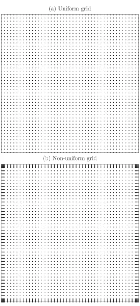
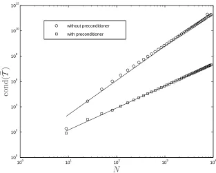
Consider a square domain [0,1]2_{. The problem domain is replaced with a Cartesian grid}

as shown in Figure 1a. Condition numbers of the transformation matrix are computed

for uniform grids, [3×3, 5 ×5, · · ·, 95 ×95]. It can be seen from Figure 2 that the preconditioned transformation system has much lower condition numbers than the original

system. At N = 9025, the proposed preconditioning scheme produces the condition number lower by about 4 orders of magnitude. The growth in the condition number is

reduced from O(N2.71_{) (unpreconditioning) to O(N}1.74_{) (preconditioning).}

To study the numerical stability of the system matrixAe, we consider the following Poisson equation

∂2_u

∂x2 1 +∂ 2_u ∂x2 2

= 4(1−π2) [sin(π(2x1 −1)) sinh(2x2−1) + 4 cosh(2(2x1−1)) cos(2π(2x2−1))],

(30)

subject to Dirichlet boundary conditions. The exact solution for this test problem is taken

as

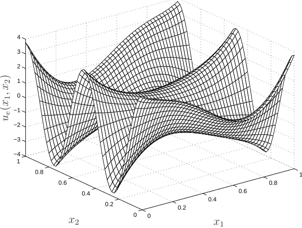
ue= sin(π(2x1−1)) sinh(2x2−1) + cosh(2(2x1−1)) cos(2π(2x2−1)). (31)

Figure 3 shows the variation of (31). To provide a basis for the assessment of the present

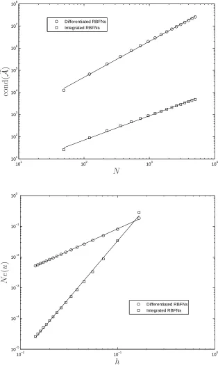
technique, we also employ conventional RBFN techniques. Conventional techniques seek

system matrix only. The field variable u is decomposed into RBFs, which are then dif-ferentiated to obtain expressions for its derivatives (difdif-ferentiated RBFNs (DRBFNs)).

We employ a set of RBFs for DRBFNs which is exactly the same as that for IRBFNs

(i.e. both approaches have the same number of RBFs, centres and widths (grid spacing)).

Grid employed are [7×7,11×11,· · · ,71×71]. Figure 4 shows that the IRBFN technique outperforms the DRBFN technique regarding both the matrix condition number and the

accuracy. It is apparent that the present system matrix is much better conditioned. The

condition number grows at the rate of O(N1.10_{) andO(N}1.62_{) for IRBFNs and DRBFNs,}

respectively. At N = 5041, the gap is about 4 orders of magnitude between the two RBF techniques (i.e. 4.89×103 _{for IRBFNs and 2.58×10}7 _{for DRBFNs). In terms of}

accuracy, the integral and differential RBF techniques yield a convergence rate ofO(h3.73₎

and O(h1.43_{) (h-the grid size), respectively.}

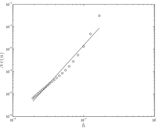
Since IRBFNs do not require an underlying grid, the present method can also work with

a non-uniform Cartesian grid. Such a discretisation is shown in Figure 1b. We employ

several non-uniform grids, namely [13×13,15×15,· · · ,59×59]. The IRBFN solution converges apparently asO(h3.49_{), wherehis the grid size of the interior region (Figure 5).}

Given a number of nodes (e.g. N = 3481), the case of using a non-uniform grid is more accurate than that of a uniform grid (e.g. 6.48×10−6 versus 5.01×10−5 for N e(u)).

3.1.2 Non-rectangular domain

The domain of interest is a circular domain of radius 1/2. The governing equation and

the exact solution are respectively taken as

∂2_u

∂x2 1

+∂

2_u

∂x2 2

= 4(1−π2) [sin(2πx1) sinh(2x2) + 4 cosh(4x1) cos(4πx2)], (32)

This problem has the same exact solution as the previous one, except that the centre of

the domain is shifted from (1/2,1/2) to (0,0). The problem domain is embedded in a

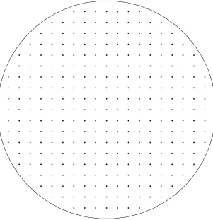
uniform Cartesian grid and the exterior grid nodes are removed (Figure 6). We generate

boundary nodes through the intersection of the grid lines and the boundary. It can be

seen that there may be some interior grid nodes that are very close to the boundary. We

introduce a parameter ∆ to study their effect on the solution accuracy. Interior nodes,

which fall within a small distance ∆ to the boundary, will be set aside. Values of ∆ are

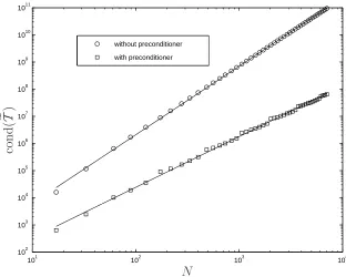
chosen here as h/4, h/6 and h/8, where h is the grid size. In Figure 7, we show a plot of the condition number of the transformation matrix versus the number of grid points.

It can be seen that the preconditioned system has a much lower condition number. Its

rate is reduced fromO(N2.52_{) (unpreconditioning) toO(N}1.86_{) (preconditioning). Table 1}

shows the condition number of the system matrix and the solution accuracy for different

values of ∆. Calculations are carried out for uniform grids, [7×7,13×13,· · ·,61×61]. It is apparent that ∆ only has a little effect on N e(u) and cond(Ae). At ∆ = h/8, the present technique yields a fast rate of convergence of O(h4.14_{) with the matrix condition}

number being in the range of 4.72×101 _{to 4.38×10}3_.

3.2

Implementation of Neumann boundary conditions on

non-rectangular boundaries

In the context of Cartesian-grid techniques, Neumann boundary conditions are known to

be more difficult to handle than Dirichlet boundary conditions. It is particularly acute

for the case of non-rectangular boundaries. It should be pointed out that the present

approximations are constructed globally through basis functions that are defined in both

x1 and x2 directions and they do not require an underlying mesh. As a result, the field

variable and its derivatives can be evaluated at any point within the domain and on its

straightforward implementation of Neumann boundary conditions on irregular boundaries.

We consider a domain with a curved boundary that is prescribed with gradient boundary

condition (Figure 8). This curve is an arc, centered at the origin, from 0 to 900 _{with a}

radius of 1/2. The top and right sides of the domain have a unit length. The governing

equation and the exact solution are taken to be the same as those used in the first example

(i.e. (30) and (31)).

As mentioned earlier, boundary points are generated by the intersection of the grid lines

and the boundaries. At boundary points created via the xj grid lines, the values of

∂2_u/∂x2

j and ∂u/∂xj are directly obtained from the networks associated withxj (they are nodal values), while the values of ∂2_u/∂x2

k and ∂u/∂xk (k 6= j) are computed from the networks associated withxk through interpolation.

A distinguishing feature of IRBFNs is that a set of their coefficients is larger owing to the

presence of integration constants. The Neumann boundary conditions can be imposed

in the final system or in the transformation system. A detailed implementation of the

two approaches for 1D-IRBFNs was presented in [24]. The latter is adopted here and its

implementation is similar to that for 1D-IRBFNs. In contrast to 1D-IRBFNs, 2D-IRBFNs

do not require the boundary points be grid nodes. Consider the xj network and let Nbj be the number of boundary points that are specified with gradient boundary condition.

Collocating the governing equation at the grid points and ∂u/∂xj at the boundary points of Neumann boundary condition, one has

e T       e w b C1 b C2      =    _cue

∂u ∂xj   =  

 eu

1

nj

c∂u

∂n −nkc ∂u ∂xk

 

, (34)

dimensions (N+Nbj)×(N+2Nk) withTeli =H

(i)

(x(l)) for 1≤l ≤N and 1≤i≤(N+2Nk) and Teli = H(i)(x

(l)

b ) for (N + 1) ≤ l ≤ (N +Nbj) and 1 ≤ i ≤ (N + 2Nk). In (34), derivative boundary conditions are forced to be satisfied exactly. The 2D-IRBFN system

thus contains information about Neumann boundary condition.

Condition numbers and errors are listed in Table 2. It can be seen that the present

technique yields a fast rate of convergence. However, solutions to Neumann

boundary-value problems are less stable than those to Dirichlet ones.

3.3

Implementation of high-order control-volume discretisations

for non-rectangular domains

Consider a second-order PDE that involves the diffusive term only

∂2_u

∂x2 1

+∂

2_u

∂x2 2

= 0, (35)

on a circular domain of radius 1/2 centered at the origin, subject to Dirichlet boundary

conditions. The exact solution is taken as

ue(x1, x2) =

1 sinh(π)sin

πx1+

π

2

sinhπx2 +

π

2

, (36)

whose variation on [−1/2,1/2]2 _{is shown in Figure 9. The problem domain is represented}

by a Cartesian grid and each interior grid node is associated with a control volume defined

by the x1 and x2 lines through the middle points of the grid node and its neighbours

(Figure 10). For grid nodes adjacent to the boundary, relevant boundary points are used

Integrating (35) over the ith control volume and applying the divergence theorem lead to

Z

Γi

∂u ∂xdy−

∂u ∂ydx

= 0, (37)

where Γi is the boundary of the control volume i. The field variable is represented by 2D-IRBFNs. The system of algebraic equations is generated by applying (37) to every

interior grid node. We will study what effect the evaluation of integrals in (37) has on the

solution accuracy. Two schemes, namely the midpoint rule and Gaussian quadrature with

5 points, are employed. To provide a basis for comparison, a control-volume approach

described in [27] is also implemented. This approach, where the gradients are represented

by linear functions and the boundary integrals are evaluated using the midpoint rule, is

referred here as linear CVM.

Figure 11 and Table 3 show results obtained by linear-CVM (middle-point rule),

IRBFN-CVMa (middle-point rule) and IRBFN-CVMb (5-point Gaussian quadrature). It is known

that the middle-point rule is only an O(h2_{) method. One thus expects that}

IRBFN-CVMa is second-order accurate. As shown in Figure 11, although more accurate, the

rate of IRBFN-CVMa is similar to that of linear-CVM. On the other hand, 5-point

Gaus-sian quadrature isO(h10_{) and the IRBFN-CVMb, as expected, outperforms linear-CVM}

and IRBFN-CVMa. In terms of cond(Ae), IRBFN-CVMa has a slightly-larger condi-tion number than linear-CVM and IRBFN-CVMb. The linear-CVM, IRBFN-CVMa and

IRBFN-CVMb have respectively their observed rates as O(N1.05_),O(N1.09_{) andO(N}1.06₎

for the condition number and O(h1.96_{), O(h}2.10_{) and O(h}3.73_{) for the solution accuracy.}

Comparing Table 3 with Table 1, it can be seen that the present control-volume approach

is less sensitive to the parameter ∆ than the present collocation approach. For all values

3.4

Discussion

2D-IRBFNs have some strengths: (i) they allow the use of high-order integration schemes

in the CV approach irrespective of the shape of the problem domain, and (ii) they have the

ability to implement Neumann boundary conditions on irregular boundaries in a direct

manner. However, the cost to construct 2D-IRBFNs is expensive. To alleviate this

draw-back, one can incorporate 1D-IRBFNs into the present Cartesian-grid numerical scheme.

For rectangular regions, 1D-IRBFNs also permit the field variable and its derivatives to

be evaluated at any point in the domain, and therefore one can use Gaussian quadrature

for the control-volume formulation. The domain of complicated shape can thus be

parti-tioned into a number of subdomains through a set of lines that are parallel to thex1 and

x2 axes; one can then employ 2D- and 1D-IRBFNs to represent the solution in irregular

and regular subdomains, respectively.

This domain decomposition procedure, which selectively exploits strengths of 1D- and

2D-IRBFNs, is numerically studied here through the domain shown in Figure 12. The

geometry of Subdomain 1 is exactly the same as that used in Section 3.2, while Subdomain

2 is a unit square. Consider a Poisson equation with Dirichlet boundary conditions. The

exact solution is created by making a simple coordinate transformation for (31) from

[0,1]2 _{to [0,2]×[0,1]. We employ a control-volume approach with 5 Gaussian points to}

discretise the governing equation on each subdomain. The two subdomains are replaced

with uniform rectangular grids of the same density. Subdomains 1 and 2 are handled

with 2D- and 1D-IRBFNs, respectively. On the interface, the values of u at the interior points are taken as unknowns and they are found using continuity of the first-order normal

derivative of the solution across the interface (the substructuring technique). Figure 13

are consistently reduced with decreasing grid size; these solutions converge apparently as

O(h3.70_).

4

CONCLUDING REMARKS

This paper is concerned with the use of 2D-IRBFNs in the context of

Cartesian-grid-based discretisation schemes for irregular domains. Some strengths and weaknesses of

2D-IRBFNs are discussed. 2D-IRBFNs have advantages in dealing with issues which

require information on the field variable and its derivatives at points that do not coincide

with regular grid nodes. Examples include the implementation of a Neumann boundary

condition on irregular boundary and the use of high-order integration schemes in the

control-volume framework. However, 2D-IRBFNs have higher matrix condition number

and require more computational effort to construct than 1D-IRBFNs. For the former, an

effective preconditioning scheme is developed. For the latter, a hybrid scheme is proposed,

where 1D-IRBFNs are incorporated into the present Cartesian-grid procedure resulting

in a much better computational efficiency. Numerical results indicate that there is a

significant improvement in matrix condition number over convention RBFN methods,

and very accurate results are achieved using relatively-coarse grids.

Acknowledgement

This work is supported by the Australian Research Council. We would like to thank the

referees for their helpful comments.

References

1. F. G. Blottner, and P. J. Roache, Nonuniform mesh systems, Journal of

2. G. H. Shortley, and R. Weller, The numerical solution of Laplace’s equation, Journal

of Applied Physics 9 (1938), 334–344.

3. Z. Jomaa, and C. Macaskill, The embedded finite difference method for the Poisson

equation in a domain with an irregular boundary and Dirichlet boundary conditions,

Journal of Computational Physics 202(2) (2005), 488–506.

4. H. Johansen, and P. Colella, A Cartesian grid embedded boundary method for

Poisson’s equation on irregular domains, Journal of Computational Physics 147(1)

(1998), 60–85.

5. P. Schwartz, M. Barad , P. Colella, and T. Ligocki, A Cartesian grid embedded

boundary method for the heat equation and Poisson’s equation in three dimensions,

Journal of Computational Physics 211(2) (2006), 531–550.

6. R. V. Viswanathan, Solution of Poisson’s equation by relaxation method–normal

gradient specified on curved boundaries, Mathematical Tables and Other Aids to

Computation 11(58) (1957), 67–78.

7. V. Thuraisamy, Approximate solutions for mixed boundary value problems by

finite-difference methods, Mathematics of Computation 23(106) (1969), 373–386.

8. V. Thuraisamy, Monotone type discrete analogue for the mixed boundary value

problem, Mathematics of Computation 23(106) (1969), 387–394.

9. E. Sanmiguel-Rojas, J. Ortega-Casanova, C. del Pino, and R. Fernandez-Feria, A

Cartesian grid finite-difference method for 2D incompressible viscous flows in

irreg-ular geometries, Journal of Computational Physics 204(1) (2005), 302–318.

10. T. J. Moroney, and I. W. Turner, A finite volume method based on radial basis

functions for two-dimensional nonlinear diffusion equations, Applied Mathematical

11. G. E. Fasshauer, Meshfree Approximation Methods With Matlab (Interdisciplinary

Mathematical Sciences - Vol. 6), World Scientific Publishers, Singapore, 2007.

12. B. Sarler, and R. Vertnik, Meshfree explicit local radial basis function collocation

method for diffusion problems, Computers & Mathematics with Applications 51(8)

(2006), 1269–1282.

13. Y. V. S. S. Sanyasiraju, and G. Chandhini, Local radial basis function based gridfree

scheme for unsteady incompressible viscous flows, Journal of Computational Physics

227(20) 2008, 8922-8948.

14. M. S. Ingber, C. S. Chen, and J. A. Tanski, A mesh free approach using radial

basis functions and parallel domain decomposition for solving three-dimensional

diffusion equations, International Journal for Numerical Methods in Engineering

60(13) (2004), 2183–2201.

15. J. Li, and Y.C. Hon, Domain decomposition for radial basis meshless methods,

Numerical Methods for Partial Differential Equations 20 (2004), 450–462.

16. E. Divo, and A. Kassab, Iterative domain decomposition meshless method modeling

of incompressible viscous flows and conjugate heat transfer, Engineering Analysis

with Boundary Elements 30(6) (2006), 465–478.

17. L. Ling, and E. J. Kansa, Preconditioning for radial basis functions with domain

decomposition methods, Mathematical and Computer Modelling 40(13) 2004, 1413–

1427.

18. H. Wendland, Error estimates for interpolation by compactly supported radial basis

functions of minimal degree, Journal of Approximation Theory 93(2) (1998), 258–

272.

19. C. S. Chen, M. Ganesh, M. A. Golberg, and A. H. -D. Cheng, Multilevel compact

& Mathematics with Applications 43(3-5) (2002), 359–378.

20. N. Mai-Duy, Solving high order ordinary differential equations with radial basis

function networks, International Journal for Numerical Methods in Engineering 62

(2005), 824–852.

21. N. Mai-Duy, and T. Tran-Cong, Solving biharmonic problems with scattered-point

discretisation using indirect radial-basis-function networks, Engineering Analysis

with Boundary Elements 30(2) (2006), 77–87.

22. N. Mai-Duy, and T. Tran-Cong, A multidomain integrated-radial-basis-function

col-location method for elliptic problems, Numerical Methods for Partial Differential

Equations 24(5) (2008), 1301–1320.

23. N. Mai-Duy, and R. I. Tanner, A collocation method based on one-dimensional RBF

interpolation scheme for solving PDEs, International Journal of Numerical Methods

for Heat & Fluid Flow 17 (2007), 165–186.

24. N. Mai-Duy, and T. Tran-Cong, A Cartesian-grid collocation method based on

radial-basis-function networks for solving PDEs in irregular domains, Numerical

Methods for Partial Differential Equations 23 (2007), 1192–1210.

25. N. Mai-Duy, and T. Tran-Cong, A control volume technique based on integrated

RBFNs for the convection-diffusion equation, Numerical Methods for Partial

Dif-ferential Equations (accepted).

26. N. Mai-Duy, and T. Tran-Cong, An efficient indirect RBFN-based method for

nu-merical solution of PDEs, Nunu-merical Methods for Partial Differential Equations 21

(2005), 770–790.

27. S. V. Patankar, Numerical Heat Transfer and Fluid Flow, McGraw-Hill, New York,

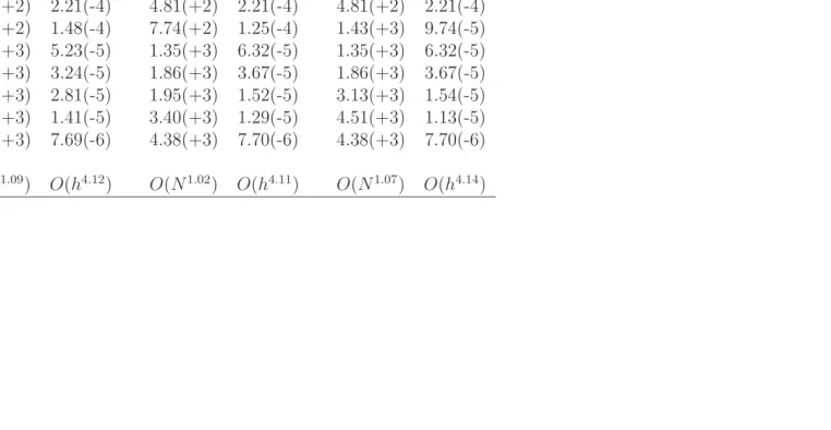
Table 1: Non-rectangular, point-collocation approach: Conditioner numbers of the system matrix and errors of the solutionu. It is noted that a(b) denotes a×10b_.

Grid ∆ =h/4 ∆ =h/6 ∆ = h/8

cond(Ae) N e(u) cond(Ae) N e(u) cond(Ae) N e(u) 7×7 2.08(+1) 1.94(-1) 4.72(+1) 1.18(-1) 4.72(+1) 1.18(-1) 13×13 1.12(+2) 3.18(-3) 1.76(+2) 5.15(-3) 1.76(+2) 5.15(-3) 19×19 2.65(+2) 8.39(-4) 2.65(+2) 8.39(-4) 2.65(+2) 8.39(-4) 25×25 4.81(+2) 2.21(-4) 4.81(+2) 2.21(-4) 4.81(+2) 2.21(-4) 31×31 7.58(+2) 1.48(-4) 7.74(+2) 1.25(-4) 1.43(+3) 9.74(-5) 37×37 1.09(+3) 5.23(-5) 1.35(+3) 6.32(-5) 1.35(+3) 6.32(-5) 43×43 1.49(+3) 3.24(-5) 1.86(+3) 3.67(-5) 1.86(+3) 3.67(-5) 49×49 1.95(+3) 2.81(-5) 1.95(+3) 1.52(-5) 3.13(+3) 1.54(-5) 55×55 2.48(+3) 1.41(-5) 3.40(+3) 1.29(-5) 4.51(+3) 1.13(-5) 61×61 3.06(+3) 7.69(-6) 4.38(+3) 7.70(-6) 4.38(+3) 7.70(-6)

O(N1.09_{) O(h}4.12_{) O(N}1.02_{) O(h}4.11_{) O(N}1.07_{) O(h}4.14₎

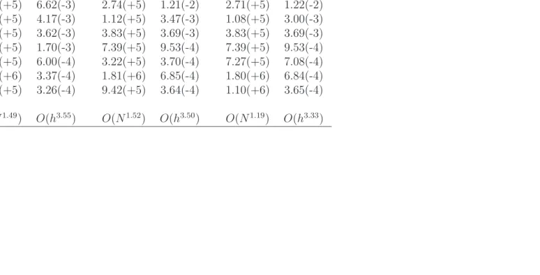
Table 2: Non-rectangular, point-collocation approach, Neumann boundary condition: Conditioner numbers of the system matrix and errors of the solution u. It is noted that a(b) denotes a×10b_.

Grid ∆ =h/4 ∆ =h/6 ∆ =h/8

cond(Ae) N e(u) cond(Ae) N e(u) cond(Ae) N e(u) 7×7 2.27(+3) 2.34(+0) 2.27(+3) 2.34(+0) 2.77(+4) 1.72(+0) 13×13 5.97(+3) 2.86(-2) 5.97(+3) 2.86(-2) 5.97(+3) 2.86(-2) 19×19 3.80(+4) 2.32(-2) 6.22(+4) 1.24(-2) 6.22(+4) 1.24(-2) 25×25 1.43(+5) 6.62(-3) 2.74(+5) 1.21(-2) 2.71(+5) 1.22(-2) 31×31 2.29(+5) 4.17(-3) 1.12(+5) 3.47(-3) 1.08(+5) 3.00(-3) 37×37 3.84(+5) 3.62(-3) 3.83(+5) 3.69(-3) 3.83(+5) 3.69(-3) 43×43 4.15(+5) 1.70(-3) 7.39(+5) 9.53(-4) 7.39(+5) 9.53(-4) 49×49 3.09(+5) 6.00(-4) 3.22(+5) 3.70(-4) 7.27(+5) 7.08(-4) 55×55 1.32(+6) 3.37(-4) 1.81(+6) 6.85(-4) 1.80(+6) 6.84(-4) 61×61 7.86(+5) 3.26(-4) 9.42(+5) 3.64(-4) 1.10(+6) 3.65(-4)

O(N1.49_{) O(h}3.55_{) O(N}1.52_{) O(h}3.50_{) O(N}1.19_{) O(h}3.33₎

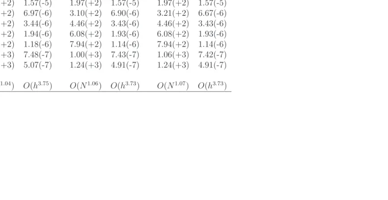
Table 3: Non-rectangular, control-volume approach, IRBFN-CVMb: Conditioner numbers of the system matrix and errors of the solutionu. It is noted that a(b) denotes a×10b_.

Grid ∆ =h/4 ∆ =h/6 ∆ = h/8

cond(Ae) N e(u) cond(Ae) N e(u) cond(Ae) N e(u) 7×7 1.16(+1) 2.85(-3) 1.13(+1) 2.61(-3) 1.13(+1) 2.61(-3) 13×13 5.10(+1) 2.17(-4) 4.85(+1) 2.08(-4) 4.85(+1) 2.08(-4) 19×19 1.10(+2) 4.70(-5) 1.10(+2) 4.70(-5) 1.10(+2) 4.70(-5) 25×25 1.97(+2) 1.57(-5) 1.97(+2) 1.57(-5) 1.97(+2) 1.57(-5) 31×31 3.14(+2) 6.97(-6) 3.10(+2) 6.90(-6) 3.21(+2) 6.67(-6) 37×37 4.48(+2) 3.44(-6) 4.46(+2) 3.43(-6) 4.46(+2) 3.43(-6) 43×43 6.09(+2) 1.94(-6) 6.08(+2) 1.93(-6) 6.08(+2) 1.93(-6) 49×49 8.77(+2) 1.18(-6) 7.94(+2) 1.14(-6) 7.94(+2) 1.14(-6) 55×55 1.00(+3) 7.48(-7) 1.00(+3) 7.43(-7) 1.06(+3) 7.42(-7) 61×61 1.32(+3) 5.07(-7) 1.24(+3) 4.91(-7) 1.24(+3) 4.91(-7)

O(N1.04_{) O(h}3.75_{) O(N}1.06_{) O(h}3.73_{) O(N}1.07_{) O(h}3.73₎

(a) Uniform grid

(b) Non-uniform grid

100 101 102 103 104 100

102 104 106 108 1010 1012

without preconditioner

with preconditioner

N

co

n

d

(

eT)

0

0.2 0.4

0.6 0.8

1

0 0.2 0.4 0.6 0.8 1 −4 −3 −2 −1 0 1 2 3 4

ue

(

x1

,x

2

)

x1

x2

Figure 3: Functionue(x1, x2) = sin(π(2x1−1)) sinh(2x2−1)+cosh(2(2x1−1)) cos(2π(2x2−

101 102 103 104 101

102 103 104 105 106 107 108

Differentiated RBFNs Integrated RBFNs

N

co

n

d

(

eA)

10−2 10−1 100

10−5 10−4 10−3 10−2 10−1 100

Differentiated RBFNs Integrated RBFNs

h

N

e

(

u

)

Figure 4: Rectangular domain, point-collocation approach: Condition numbers of the system matrix and errors of the solution by IRBFNs and DRBFNs. The values of N

10−2 10−1 100 10−6

10−5 10−4 10−3 10−2 10−1

h

N

e

(

u

)

101 102 103 104 102

103 104 105 106 107 108 109 1010 1011

without preconditioner

with preconditioner

N

co

n

d

(

eT)

Figure 7: Non-rectangular domain, ∆ = h/4: Condition numbers of the transformation matrix versus the total number of nodal points. Grids employed are [5×5,7×7,· · · ,95×

∂u/∂n

u

u u

u

−0.5

0

0.5

−0.5 0

0.5 0 0.2 0.4 0.6 0.8 1

ue

(

x1

,x

2

)

x1

x2

101 102 103 104 100

101 102 103 104

Linear−CVM IRBFN−CVMa IRBFN−CVMb

N

co

n

d

(

e_A)

10−2 10−1 100

10−7 10−6 10−5 10−4 10−3 10−2 10−1

Linear−CVM IRBFN−CVMa IRBFN−CVMb

h

N

e

(

u

)

Subdomain 1

Subdomain 2

100 101 102 100

101 102

Nf

co

n

d

(

b_A)f

10−2 10−1 100

10−5 10−4 10−3 10−2 10−1 100 101

Subdomain 1

Subdomain 2

Whole domain

h

N

e

(

u

)