On-line distributed hierarchical control and optimisation of large scale systems

City, University of London Institutional Repository

Citation: Li, C.W. (1990). On-line distributed hierarchical control and optimisation of large scale systems. (Unpublished Doctoral thesis, City University London)

This is the accepted version of the paper.

This version of the publication may differ from the final published version.

Permanent repository link: http://openaccess.city.ac.uk/7528/

Link to published version:

Copyright and reuse: City Research Online aims to make research outputs of City, University of London available to a wider audience. Copyright and Moral Rights remain with the author(s) and/or copyright holders. URLs from City Research Online may be freely distributed and linked to.

City Research Online: http://openaccess.city.ac.uk/ [email protected]

On-Line Distributed Hierarchical control and optimisation of Large Scale Systems

By

Chung Wai LI

Thesis submitted for the award of the degree of

Doctor of Philosophy

City University London

Control Engineering Centre

BEST COpy

AVAILABLE

TEXT IN ORIGINAL

IS

1.

2.

3 .

CONTENTS

ACKNOWLEDGEMENTS

DECLARATION

ABSTRACT

SYMBOLS AND/OR ABBREVIATIONS

Introduction

Hierarchical Control and Optimisation of Large Scale

Systems

2.1 Introduction

2.2 Basic Types of Hierarchical Structure

Page

5

6

7

8

9

14

14

15

2.2.1 Multi-strata Hierarchical Structure 16

2.2.2 Multi-layer Hierarchical Structure 18

2.2.3 Multi-echelon (Multi-level) Hierarchical 21

Structure

2.3 Coordination Methods

2.3.1 Interaction Prediction Method (IPM)

2.3.2 Interaction Balance Method (IBM)

2.4 Optimisation Methods

2.5 Summary

Distributed Hierarchical Computer System (DHCS)

3.1 Introduction

3.2 Coordinator (LSI-11/23)

3.3 Local Decision unit (I-MIC)

3.4 Simulated Interconnected ·Process (TR48)

3.5 Summary

24

25

26

27

28

29

29

31

32

33

4 •

5.

6.

Formulation of Control Problem

4.1 Control Problem Formulation

35

35

4.2 Mathematical Model of the Hierarchical Control 40

structure

4.3 Summary 41

On-line Coordination methods

5.1 Introduction

42

42

5.2 Closed-loop Coordination Methods 42

5.2.1 Interaction Prediction Method with Global 43

Feedback (IPMGF)

5.2.2 Interaction Prediction Method with Local 44

Feedback (IPMLF)

5. 2 . 3 Interac::'ion Balance Method with Global 47

Feedback (IBMGF)

5. 2 . 4 Interaction Balance Method with Local

Feedback (IBMLF)

48

5.3 Synchronisation and Interprocess Communication 51

5.4 Asynchronous Iteration for Closed-loop 53

Hierarchical control and Optimisation of

Interconnected Systems

5.5 Summary

Software Development

6.1 Introduction

6.2 Coordinator (LSI-11/23) Software

6.2.1 Program Units

6.2.1.1 Foreground Routines

6.2.1.2 Background Rountines

6.2.1.2.1 Main Program

6.2.1.2.2 Subroutine IBMF23

6.3 Local Decision unit (I-MIC) Software

6.4 Simulated Interconnected Process

6.5 Summary

3

55

57

57

57

58

60

60

61

63 63

68

7 .

8.

simulation Results and Discussion

7.1 Introduction

71

71

72

7.2 Synchronous Local Decision Iteration

7.2.1 Interaction Prediction with Global Feedback 72

7.2.2 Interaction Prediction with Local Feedback 76

7.2.3 Interaction Balance with Global Feedback 77

7.2.4 Interaction Balance with Local Feedback 79

7.3 Asynchronous Local Decision Iteration 81

7.3.1 Interaction Prediction with Local Feedback 81

7.3.2 Interaction Balance with Local Feedback

7.4 Summary of Simulation Results

83

85

86

7.5 Graphical Output of Simulation Results

Conclusions 105

References and Bibliography 109

Appendices 115

A. Local Decision Feasibility set under Constraints 115

B. Coordinator (LSI-11/23) Software Listings 120

C.

B1. Foreground Routines 120

B2. Background Routines 130

B2.1 Interaction Balance with Local Feedback 130

B2.2 Interaction Balance with Global Feedback 147

B2.3 Interaction Prediction with Local Feedback 160

B2.4 Interaction Prediction with Global Feedback 173

Local Decision units (I-MICs) Software Listings 188

C1. Interaction Prediction with Global Feedback 188

C2. Interaction Prediction with Local Feedback 198

C3. Interaction Balance with Global Feedback 207

ACKNOWLEDGEMENTS

I would like to express my greatest appreciation to

my project supervisor, Professor P.D. Roberts for his

inval uable adv ice, guidance and support throughout the

course of my research.

I am also indebted to Mr. D. S . Wadhwani, Dr. I. A.

Stevenson and Dr. J.E. Ellis for their help and valuable discussions in the Computer Control Laboratory.

Also, I would like to thank all members of staff and

friends in the Control Engineering Centre who have contributed to this research.

Finally, I am grateful for the financial support from

the Science and Engineering Research Council.

DECLARATION

ABSTRACT

This research is concerned with the application of closed-loop coordination techniques for on-line steady state optimisation and control of large scale systems

using a micro-computer based system. A two-level

hierarchical computer structure consisting of a

coordinator at the supremal (upper) level and two local decision units at the infimal (lower) level had been

established. Parallel computation were performed at the

local decision unit level once the coordination parameters had been received from the supremal level. A steady state

system model consisting of two interconnected

subprocesses, simulated oy an analogue computer, was used

to investigate the coordination methods for closed-loop

hierarchical control. First-order time constants were introduced to the interaction inputs and the controls within the simulated subprocesses.

Investigations had been carried out to study

closed-loop control using the Interaction Prediction and

Interaction Balance coordination method. Special

attention was given to the study of the problems

associated with synchronisation of the local decision units for closed-loop control. Stability aspects of both coordination methods when subjected to disturbances in the

controls and interconnections had been investigated~

Problems relating to system transient and local. decision asynchronisation, as well as their effects on system stabil i ty and convergence of the two tasks, namely the local decision task and the coordinator task had also been investigated. Methods for dealing with these problems had

been suggested. The sub-optimal i ty, convergency and

robustness properties of each coordination method had been

discussed. This research has demonstrated that the

Interaction Prediction coordination methods are best suited for on-line distributed optimising control of large scale interconnected systems. Using the local feedback scheme, complete decentralisation at the local decision level operated asynchronou.sly can be achieved with the Interaction Prediction coordination method.

c COP DHCS

F

F.

G H

IBM IBMGF IBMLF I-MIC IPM IPMGF

IPMLF

K, (;

L,A

LDU LOP

Q

u

u.

v

y

y. z

SYMBOLS AND/OR ABBREVIATIONS

Control input

Coordinator Optimisation Problem

Distributed Hierarchical Computer System Input/output mapping (model)

Input/output mapping (real system) Constraint set

Interconnection matrix

Interaction Balance Method

Interaction Balance Method with Global Feedback Interaction Balance Method with Local Feedback Industrial MIcro-Controller

Interaction Prediction Method Interaction

Feedback

Prediction Method with Global

Interaction Prediction Method with Local Feedback System gain matrix

Lagrangian

Local Decision Unit

Local Optimisation Problem

Performance index (model)

_..

Performance index (real system) SUboptimility

Shift vector

Interaction input (model)

Interaction input (real system) Coordination variables for IPM Interaction output (model)

CHAPTER 1 INTRODUCTION

There has been a growing attention paid to the subj ect area of large scale systems. This comes quite

naturally as many real-life problems of socio-economic,

environmental and technological nature are highly complex,

large in dimension and stochastic in nature. Despite its

generali ty and usefulness, the mul tivariable system

approach is severely limited when applied to problems of high dimension and complex interconnecting structure. For

this reason it is frequently advantageous to view high

order systems as being composed of several lower order subsystems which when interconnected in an appropriate

fashion, yield the original composite or interconnected

system.

Many viewpoints have been put forward to define and

quantify a system as 'large scale'. One viewpoint

considers 'large scale systems' as those whose dimensions

are so large that conventional techniques of modelling,

analysis, control and optimisation are extremely diff~cult

or impossible to give a reasonable solution. Another

.

viewpoint suggests that if a system can be decomposed into a number of interconnected subsystems for computational

and· practical purposes, then such systems are termed as

large scale systems. The latter viewpoint is adopted to

define large scale systems.

Theoretical investigations and researches to develop conceptual framework and mathematical theory to model,

analyse and control these structured, complex, large scale

systems have been carried out since early sixties.

Basically, the main idea behind this approach is the

recognition that complex systems are structured In a

hierarchical order. This approach in fact recommends that

for a mathematical theory to claim to be dealing with

large scale complex systems, the complexity of the real

systems must be reflected in the structure of the model.

Many research papers concerning the theory and methodology

of large scale systems were published throughout the

sixties. In 1970, Mesarovic, Macho and Takahara presented

one of the earliest formal quantitative treatments of

hierarchical (multi-level) systems. Since then, a great

deal of work has been done in this field and many papers

which are based upon these theoretical works have been published and presented in many conferences from different

fields. Many researchers have addressed themselves to

various problems concerned with large scale systems.

Excellent survey papers on the topic of hierarchical

(multi-level) control and optimisation of large scale

systems were given by Mahmoud (1977), Singh (1981,1982).

Roughly speaking, problems concerned with large scale systems may be divided into two broad areas: static

problems and dynamic problems. However, this research is

focussed only on hierarchical optimisation and control of

large scale systems operating at steady state condition.

Because of economic reasons and intensive competition

within the market sector, increasing pressure is stressed

upon industry to improve efficiency and productivity of

in.dustrial plants. A method for the practical

.

implementation of an on-line optimisation and control scheme for an industrial process considers the overall

design as a two layer hierarchical system. This is a form

of optimising control where the lower layer contains

regulatory feedback controllers used to maintain the

system at a steady state operating condition specified by

controller set points. Optimisation is performed in the

upper layer, where a steady state mathematical model 1S

used to compute the optimal values of the controller set

points to maximise the operational efficiency.

Recent techniques specifically consider a large scale

industrial system as a collection of interlinked

sub-systems. Modern computer technology which has resulted in

low cost computer power may then be employed with the

advantage 1n order to employ m1cro or mini-computers,

structure, to coordinate, optimise and regulate individual

decision task and sub-process. When designed carefully

this control strategy has the advantages of reducing

computer storage and computation time accomplished through

parallel processing, increased system flexibility and

reliability, and cheap hardware cost. Furthermore, i t

identifies and organises the information flow through the

system. Thus provides effective use of feedbacks for

control and decision making process which 1.S attractive

for on-line control purposes.

Three problems associated with on-line hierarchical optimisation and control of industrial processes are

considered. Firstly, the behaviour of each process under

control lS not known and the mathematical model

representing the real process is only an approximation.

Secondly, the nature and magnitude of disturbances affecting the real process are stochastic. Lastly, timing problems arise because the real process, the sUb-system

decision units and the coordinator are processing at different speeds. One way to reduce the first two problems

is to use feedback information from real process

measurements. For timing problems, the local decision units at the infimal level should be synchronised with the

coordinator and a simple synchronisation method

"semaphore" has been used.

Since late seventies, several hierarchical control schemes have been suggested for on-line control of steady

state systems by Findeisen (1978,1979), Brdys

(1978,1979), Roberts (1983), Shao (1983). These proposed

schemes were investigated by off-line simulations of

interconnected hierarchical systems. The objective of this

research 1.S to implement some of the proposed schemes

through a distributed control system in order to

investigate the closed-loop hierarchical control of a

simulated interconnected industrial process. The on-line

closed-loop hierarchical control schemes used in this

research are the well-known Interaction Prediction Method

and the Interaction Balance Method wi th local or global

feedback. Implementation problems that may arlse for

different closed-loop hierarchical control and

optimisation of an interconnected system were examined.

study of on-line distributed hierarchical control with the

local decision units operating asynchronisely had also

been performed and implementated with the distributed

hierarchical computer system.

The major contributions of knowledge of this thesis can be summarised as follows. This is the first time that

hierarchical control algorithms (the Interaction

Prediction Method and the Interaction Balance Method with

local or global feeback) have actually been investigated

in a real-time environment. with a suitable

synchronisation scheme, parallel processing at the infimal

level within the hierarchical structure has been achieved.

This greatly reduces the computation time required by the local decision units which again reduces the overall computation time required.

Investigation of the problems relating to on-line

hierarchical control and optimisation of interconnecting

systems have been carried out. These problems are the

transfer lags, measurement errors, subprocess and decision unit failures. An analogue computer was used to simulate

these problems. The transfer lags were simulated by means

of introducing a first order time constant in the controls

and interaction variables. The measurement errors,

subprocess and decision unit failures were simulated by

varying the potentiometers wi thin the analogue computer

that correspond to the controls and the interaction

variables. The stability, convergence and the system

response of the decision problems when subjected to these

problems were examined.

Coordinated by Interaction Prediction Method and the

Interaction Balance Method with local feedback, simulation

studies had been made concerning synchronisation of

subsystem decision units and the effects of

coordinator and local decision optimisation problems.

Interaction Prediction Method with local feedback offers a

stable and converging decision problems while the

Interaction Balance Method with local feedback is very sensitive and becoming unstable when local decision units

are operating asynchronously.

CHAPTER 2 HIERARCHICAL CONTROL AND OPTIMISATION OF LARGE SCALE SYSTEMS

2.1 Introduction

Hierarchical, multi-level system theory was introduced by Mesarovic and his associates (1970) with an objective of establishing a conceptual framework to mathematical theory in order to tackle complex multi-goal decision makir.g

systems. The basic idea behind this theory lS the

recognition

that

are structured in a pyramid-like form. It lS therefore

natural to develop a mathematical model of the structural approach to control these complex systems.

Some key properties associated with hierarchical

systems can be summarised as follows:

a) The decision making units are arranged In a pyramid-like structure;

b) Information flow between varlOUS levels of hierarchy are exchanged' iteratively and (usually) vertically;

c) The objectives of local decision units may be In

conflict which have to be resolved by the coordinator:

d) Time horizon increases as the level of hierarchy goes

up;

e) Existence of a supremal unit.

the

optimisation of large

fact that there is

scale systems

a possibility

lS motivated by

of SUbstantial

economic sav ings which may happen in both the des ign and

operational phases. Both static optimisation (f ini te

dimensional) and dynamic optimisation (infinite

dimensional) techniques are involved In the control of

An essential concept of the hierarchical control and

optimisation approach for complex large scale systems

control is the consideration of the overall control system

as replaced by a set of smaller interdependent sUbsystems.

Each subsystem has to serve a particular function, shares

resources, and is governed by an interrelated objective and

a set of constraints. Subsystems which are in the lowest

(infimal) level of the hierarchy are often called infimal

or local decision units while those in the higher

(supremal) level are referred as coordinator or supremal

units. The obj ecti ves of the subsystems in the inf imal

level are then solved independently under the intervention of a coordinator in the supremal level. The task of the

coordinator is to account for the interconnections and

constraints between the infimal units such that the overall

system obj ecti ve can be represented by the collection of

individual subsystem objectives. Thus, the successful

operation of hierarchical systems is best described by two

processes: decomposition or infimal generation and

coordination or overall objective synthesis.

section 2.2 outlines the basic types of hierarchical

structures. sections 2.3 and 2.4 are concerned with

alternative methods of coordination and optimisation

respectively. Finally, a short summary is given in section

2 • 5.

2.2 Basic Types of Hierarchical structures

Based on the hierarchical systems approach, an overall

complex large scale problem may be decomposed into a

collection of interconnected smaller subproblems arranged

in a hierarchical structure. There are three basic types of

hierarchical structure (Mesarovic 1970), namely,

1) Multi-strata hierarchical structure;

2) Multi-layer hierarchical structure;

3) Multi-echelon (Multi-level) hierarchical structure.

The classification of these hierarchical structures is

based on the decomposition criterion chosen for the overall

complex problem. It should be noted that many real-life complex systems may belong to more than one class of these

hierarchical structures. Also, the operation of each of

these types of hierarchy depends heavily on the information

exchange mechanism between adj acent levels, the explicit

specification of the subproblems and their objectives, and

the proper manipulation of the subsystems activities. The

hierarchical structures and their characteristics will be

outlined in the following sUbsections.

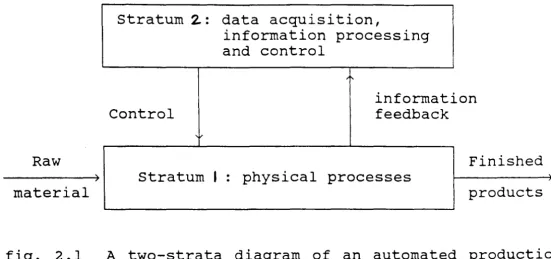
2.2.1 Multi-strata Hierarchical structure

The multi-strata type of hierarchical structure

describes the system by a family of models each concerned

with the behaviour of the system as viewed from a different level of abstraaion. The levels of this type of structure

are often called strata. For each level, there is a set of

relevent features and variables, laws and principles in

terms of which the behaviour of the system is described. It

is necessary that the functioning on any level be as

independent as possible of the functioning on other levels.

The partitioning into strata has the objective of

simplifying the overall complex problem by separating the

problem into a number of smaller, better defined

subproblems each of which is solved separately.

Let us illustrate the stratified description of a

hierarchical structure by an automated production process

Raw

)

material

fig. 2. I

stratum 2: data acquisition,

information processing and control

Control

information feedback

Finished

stratum I : physical processes

products

A two-strata diagram of an automated production

process

These strata are used to deal with the same item, i.e.

the finished product. On the first stratum, the.product is

viewed as a physical obj ect to be changed in accordance

with physical laws. On the second stratum which deals with data acquisition, information processing and control, the same item is viewed as a variable to be controlled and

manipulated. A different model is used for each of these

views of the system.

A Multi-strata hierarchical structure has the

following characteristics,

a) The selection of strata depends upon the observer, his

knowledge and interest in the operation of the system;

b) In general, contexts in which the operation of a system

on different strata described are not mutually related;

the principles used to describe the system on any

stratum cannot generally be derived from the principles

used on other strata;

c) There exists an interdependence between the

functioning of a system on different strata;

d) Comprehension of a system increases by crosslng

.

strata: the lower strata are assigned with more detailed

and specialised descriptions while higher strata have a

deeper understanding of its significance.

Decomposition on the basis of stratum is not based on

the decomposition of a well-formulated mathematical

programming problem. Therefore, there is no rigorous theory

to justify its performance. This method partitions the

control problem in such a way that it can be solved

sequentially in strata with the result of one stratum

serving as partial input to the other stratum below. Thus

the decision making process possesses the characteristics

of a staged process rather than those of a completely

interacting one.

2.2.2 Multi-layer Hierarchical structure

Mul ti-layer description of a hierarchical system 1S

concerned with levels of decision complexity. The levels of this hierarchy are called layers. Essentially, the idea

behind this hierarchical approach is that one defines a set

of control problems whose solution is attempted 1n a

sequentially manner. The overall control problem is

substituted by a set of sequentially arranged simpler

subproblems so that the solution of all the subproblems in

the set implies the sclutionof the original problem. Within the hierarchy each layer operates at different time

horizons, therefore, multi-layer description may be viewed

as vertical decomposition of control structures.

Multi-layer hierarchical system may further be divided into

two different classes depending on the decomposition

criteria, these are:

a) Functional multi-layer structure decomposition

according to control function;

b) Temporal multi-layer structure decomposition

according to time scale.

As an example of functional mul ti-layer hierarchies,

we consider a functional four-layer control hierarchy under

uncertainties. The four functional control layers are,

self-organisation.

A schematic diagram of a functional four-layer control structure is shown in fig 2.2.

Self organisation

v

Adaptation

,,,

v

optimisation

Regulation

,

,l,-) Industrial process

Flq.2.2 schematIc diagram of a fU[lctioIlal four-layer control structure

Now let us look into the functional aspects of each

layer within the hierarchy.

First layer: This is the regulation or direct control

layer whose task is to maintain the process

variables at prescribed set-point values

under the influence of disturbances. This

layer incorporates the functions of data

acquisition, event monitoring and

control.

direct

Second layer: The optimisation or supervisory layer whose

objective is to specify set-point values for

the regulation layer. The set-point values

are determined by optimising a mathematical

model which approximates the real process

under control.

Third layer: The adaptation or learning layer is concerned

with specifying or updating the uncertain

parameters of the mathematical model used by

the supervisory layer in order to simplify

the task of the second layer.

Fourth layer: The self-organising layer whose task 1S to

select the structure, functions and

strategies which are used on the lower layers

so that an overall objective is being pursued

as closely as possible. It can

parameters of the models used by

layers if either the control

unsatisfactory or the overall goal

The characteristics of a functional

hierarchical structure are:

a) A natural hierarchy in which each layer has a

of action over the layer below;

change the

the lower

action 1S

changes.

multi-layer

priority

b) The layers of the hierarchy represent different kinds of control functions, therefore, require different kinds of

information processing and computation algorithms;

c) The layers of the hierarchy can be designed to respond

to disturbance inputs having different frequency

characteristics.

Thus, functional multi-layer hierarchical approach

provides a rational and systematic procedure for resolving

complex large scale problems.

For temporal multi-layer control structure, the

partition of the control problem into subproblems is based

on different time scales relevant to the associated action

(a) Minimum information acquisition time;

(b) Bandwidth properties or mean time between discrete

changes in disturbance inputs;

(c) Minimum time horizon associated with the control

action;

(d) Cost-benefit trade-off considerations.

Within a temporal multi-layer control structure, the . th 1

1 ayer controller generates a control action, on an

average, every T seconds, with T > T

i i +1 i ' i=1,2, .. , based

on

(a) Current input information;

(b) Targets and/or constraints provided by a

layer controller;

(i+1) th

(c) Feedback information provided by a (k_1)th controller.

The advantages of using temporal multi-layer

decomposition approach for large scale system analysis are:

(a) Reducing the effects of uncertainty;

(b) Introduction of feedback of experience;

(c) Aggregating variables and simplifying ~odels;

(d) Implementing systems integration through well-defined

assignments of tasks and responsibilities.

An example of a temporal multi-layer structure

considers a mUlti-time scale production planning and

scheduling system whereby the planning may be on a yearly plan, monthly plan, daily schedule etc. Therefore each

layer of the hierarchy generates the targets/constraints

for the layer below and tries to maintain the prior plan or

schedule using the feedback information.

2.2.3 Multi-echelon (Multi-level) Hierarchical structure

This is the most general type of hierarchy which uses

a structural or organisational approach to decouple a

system. _{The basis of this hierarchical decomposition}

considers the partitioning of a system into separate

subsystems each with its own and perhaps conflicting goals and interaction among the subsystems. The subsystems are

positioned on different levels wi thin the hierarchy such

that each one can coordinate lower level units and be

coordinated by a higher level one. Each subsystem pursues

its own assigned goal independently. Since the subsystems

are coupled and interacting, a higher level uni t

(coordinator) is used to coordinate the subsystems in the

lower level to account for the disturbances introduced by

the interacting sUbsystems. The levels of this

hierarchical structure are called echelons.

Basically, there are three categories concerned with

decision making systems with respect to hierarchical

arrangements 9f decision units. They are single-level

single-goal systems, single-level mul ti-goal systems and multi-level multi-goal systems which are shown in fig.2.3.

Decision Making unit

,

'v

-" Process -"

Fig.2.3a Single-level single-goal system

Decision unit 1 I- - - Decision unit N

I'

,

....lo. Process

I

01

1

SP 1

~

?I

'"

I.C ~

02

~~

1 m

...

01 01

2 n - 1

.... ··· ... u_ .... _. ••.• . ... __ ... .

SP

2

1 . . -_ _ --1

SP

~---l n - 1 Process

D1

n

SP n

...

Fig.2.3c Multi-level multi-goal system

For single-level single-goal system, a goal is defined for the overall system, and all decision variables are selected in order to satisfy this goal. This centralised

decision making system has an advantage of conceptual

simplicity but technically it is very difficult to be

implemented for large scale complex problem.

Single-level ~ulti-goal system consists of a family of

decision units, each with its own goals. The goals are not

necessarily conflicting. This lS a decentralised decision

making system with the advantage of problem sharing.

Multi-level multi-goal system lS the general

representation of large scale system where the decision

units are arranged In a pyramid-form structure. Each level

consists of a number of decision units, each with its own

goal. Some of these decision units are coordinated by

another decision unit in the level above. There exists a

suprema 1 unit at the top level which characterised this

decision making system.

The multi-level approach for the decomposition of large scale systems has the following advantages:

(a) Reduction in development costs;

(b) Reduction in total computation effort;

(c) Reduction in data/information exchange;

(d) Increase system reliability.

2.3 Coordination Methods

In order to solve complex large scale systems, it 1S necessary to decompose the system and/or its control into a

set of smaller subsystems, and 1n addition to provide a mechanism for coordination of the subsystems so as to

achieve the overall system objective. The transformation of

a given integrated system into a hierarchical one can be

achieved by different ways as outlined in the preceding

sections. However, the problem of coordinating these

subsystems is not always straight forward and places a

practical limitation on the decomposition. This is

especially true 1n an on-line system because the response

constraint in real time may hinder many coordination

algorithms which are theoretically possible (e.g.

unfeasible methods). Therefore it is important to determine

techniques for coordination 1n each type of multi -level

structures and to consider the methods by which each

structure handles physical disturbances 1n the system

together with interaction disturbances introduced by the

decomposed nature of the system.

Coordination between the supremal and the infimal

levels within the hierarchy can be achieved by transmitting

coordination signals from the suprema 1 coordinator to each

infimal unit and, 1n turn, receives performance information

from the inf imal units. Most of coordination schemes are

Interaction Balance Method (IBM) and Interaction Prediction

Method (IPM). These coordination method are similar in the

sense that they initiate local decision optimisation

computation in the infimal level by specifying intervention

parameters from the supremal level. The method by which the

supremal level calculates the coordination parameters and

intervenes the in·fimal level defines the coordination

strategy.

In the following subsections, these coordination

methods are briefly described. A detailed treatment on

on-line coordination methods suitable for closed-loop

control and optimisation of interconnected system can be found in chapter 5.

2.3.1. _{Interaction Prediction Method (IPM)}

This coordination method lS

.

coordination, primal coordination, method of projection and parametric decomposition.

The "main feature of this method lS that the supremal

unit prescribes the interaction variables of the

sUbsystems. At each iteration, the coordinator specifies

the interaction variables, and the infimal units proceed to solve their model based local decision problems on the

assumption that the interaction variables are as exactly as

predicted by the suprema 1 unit. Based on the measurement

taken from the real process (real interaction variables)

and the solution information from the local decision units,

the coordinator employs an iterative procedure which

adjusts the specification of the interaction variables

until the global optimum lS obtained, l.e. the real

interaction variables are identical to the predicted ones.

Interaction Prediction method is inherently sui table

for on-line application since all the intermediate results

of the i terati ve optimisation can be appl ied directly to

the real process because all interconnection contraints are

always satisfied. Hence, this method 1S classified as

feasible coordination strategy.

One of the disadvantagesof this coordination method is the overdetermined subsystem optimisation problems at the

infimal level. This overdetermined problem can be eased by

either reducing the effective number of interconnections

between subsystems or relaxing the interconnection

constraints on the expense of losing the feasibility

property which this coordination method posesses. Another source of difficulty is that, 1n general, the gradient of

the objective function is not easy to compute and may not

even exist. Therefore, this 1S not really possible to solve

the coordinator problem effectively without gradient

information. Furthermore, it is important to ensure that

the coordination variables are such that the local decision

solutions lie in the feasible region within the constraint

boundaries.

2.3.2 Interaction Balance Method (IBM)

Alternative names of this coordination method are goal

coordination, price coordination and dual coordination.

This coordination method considers the

interconnections between subsystems as additional

constraints on the local optimisation problem. Sui table

modification of the infimal objective functions is made to

take account of the interactions between subsystems. A

decomposable Lagrangian may be formed to provide the

modified objective function for each subsystem optimisation

problem. The task of the coordinator 1S to select

interaction inputs to the infimal units such that all

interconnection constraints are satisf ied (i. e. In

balance). This means that the final optimum solution of the

Since _{the interconnection constraints are not}

satisfied during the early stages of the _iterative

optimisation procedure and only the final 'balanced'

solution can be applied to the real process, interaction

balance method is termed as non-feasible coordination

strategy.

Analytically, _{coordination by Interaction Balance}

Method is more appeal ing than the Interaction Prediction Method as the formulation of the former method is based on the well-known Lagrangian theory. Only mild assumptions of continuity and convexity are needed to ensure existence of

solution of the optimisation problem. If the solution of

the Lagrangian function is unique, the gradient of the dual

function exists. Then reasonably fast gradient-type

optimisation algorithm can be implemented to solve the dual

(coordinator) problem. However, if the problem lS not

convex, duality gap problem may occur. Then the solution

obtained by the dual formulation mayor may not be the correct optimum.

2.4 Optimisation Methods

Having decomposed the overall control problem into

subproblems,

and suprema 1

optimisation is performed in both the infimal

levels within the hierarchy. The local

units compute the optimal controller set-point decision

values for the subprocesses under control and the

coordinator determines the intervention parameters to

account for the constraints and interaction between

subsystems such that the overall performance requirements

are achieved.

A number of numerical methods based on mathematical

programming are available for solving these optimisation

problems. The choice of the method depends upon its

numerical properties and the nature of the problem under

investigation. The optimisation problem may be linear or

non-linear, unconstrained or constrained, mono-variable or

multi-variable. The numerical properties of an optimisation

algorithm are the existence of the numerical solution

approach, the convergence of the algorithm and computation

time required. For steady-state optimisation problems,

direct and gradient methods are commonly used for

unconstrained problems. The simplex method is ideal for

linear constrained problems. Primal and dual methods

incorporating augmented Lagrangians may be employed for

non-linear constrained optimisation problems.

Details of these optimisation algorithms are well

documented in the mathematical programming literature. Each

has its advantages and disadvantages. Enough experlence

with these numerical algorithms enables proper selection of algorithm or combination of algorithms to suit the nature

of a particular problem.

2.5 Summary

This chapter introduces the basic concept of

hierarchical control and optimisation of large scale

systems using the decomposition and coordination approach.

Decomposition of complex system into one or a mixture of the three basic types of hierarchical structure, namely,

the muti-strata, multi-layer, and multi-level, depends on

the nature of the system under study. The characteristics

of the three basic hierarchical structures have been

briefly described. Then, methods of coordinating the

decomposed system using the Interaction Prediction and the

Interaction Balance principles are briefly outlined.

Finally, a brief description of optimisation methods that

CHAPTER 3 DISTRIBUTED HIERARCHICAL COMPUTER SYSTEM (DHCS)

3.1 Introduction

within the Computer Control Laboratory of City University there is a distributed two-level hierarchical computer system. The infimal level of the hierarchy contains four I-MIC micro-computers and a LSI-11/02 mini-computer, which are used as local decision units for direct control of pilot plants and a small analogue computer system operating at steady state conditions. A DEC LSI-11/23 mini-computer with a time shared operating system is employed at the supremal level which acts as a host machine to coordinate and supervise computers (local decision units) at the lower level. There is also a BBC micro-computer system with a visual display, a disk drive

and a printer.

At present the I-MICs control a pilot scale freon vaporiser, a mixing process and simulated interconnected dynamic processes on the analogue computer. The LSI-ll/02 controls a pilot-scale eight zone electrically heated travelling load furnace. A schematic diagram of the

distributed hierarchical computer system lS shown in

fig.3.1

I II I. 2J1 bvW F l CIf>P'J

LSI II~

~

I

,. ... •

...

.-•

1tS-2:!2 _I I YOU

",.1_,50 Jt----1ACra

(I,. Lab)

I

1 - - - - / LIM ,.,.Inw.- LA II~

L 1,.t..coL .... &0810

FLoppJl 2 II . . ~.

---~ FLoppJl

-1

I

AOnl2

c...vol.

. .. 1

FIll. l .

I

YOU LSI

ACra 1 - - - 1 11,.2

::IGX1W1 1-nIC I Cl( IIlAn v.,..,...

,

..

Sc·hl~IIl .... i t i c d,,-h:{ram of tht' distributed hlt'rarchica]

computpr syst.PIll

In order to investigate the decomposi tion-coordination methods used for on-line optimisation and

control of interconnected system a two-level hierarchical

structure was established. At the infimal level of the

hierarchy two I-MIC micro-computers are used

decision units whose task is to determine the

controller set point values from a given

as local

optimal

set of coordinator intervention variables. The LSI-ll/23

mini-computer which acts as the coordinator supervises the

I-MICs in order to achieve the overall optimal solution. The

coordinator is also used to synChronise ~he local decision

units before optimal controls are applied to the simulated interconnected dynamic real process.

A EAL Pace TR48 analogue computer is used to simUlate

an interconnected dynamic real process with first order

transfer lags introduced in the controls and

interconnected inputs. The existence of disturbances and

model-reality differences cause the real process under control to deviate from its desired optimal steady state

condition. Corrective action can be made using feedback based on measurements by which the current· state of the

real process is inferred relative to an assesssment of the

desired state. Feedback information from the analogue

computer is implemented globally or locally within the

hierarchy. The two level hierarchical structure is shown

in fig.3 2

. .

COORDINATOR

LS111-23

£1

i~

LOCAL DECISION _I I LOCAL DECISION

UNIT 1 _r--~-I

L--_

I-MIC 1 _I I I-MIC 2

I I

I I

C'L. I I ClI Cu C1J

CII' _{I I}

I

I 1

I I

DIRECT CONTROL _I I DIRECT CONTROL

'ill _{J I} V 11

A brief description on the computers used as

coordinator, the local decision units and the simulated real process, i.e. the LSI-11/23, the I-MIC and the TR48, can be found in the following sections.

3.2 Coordinator ( LSI-11/23 )

The LSI-11/23 has a full complement of 256K bytes RAM

and runs the TSX-PLUS time shared operating system. It is

a general purpose time shared operating system which can provide computing facilities, both off-line and real-time,

for up to twenty users working concurrently. The TSX-PLUS

operating system is based on the DEC RT-11 single job

monitor with some extended features such as a transparent

line-printer spooling system, a shared file record locking

facility, an inter-job message communication facility, a program performance monitor system, command files with

parameters and a logon and usage accounting system. Such

features greatly enhance the system performance,

particularly in real-time applications. Having logged on, each user is allocated with 20K bytes of memory which can

be extended up to 56K bytes. This is more than the

~previous single job operating system RT-11 can provide.

Programs and data are stored on two 2 OM bytes

Winchester disks and a 1.2M bytes floppy disk drive. The

peripherals which are available to the LSI-11/23 include

one ADM5 and two ADM22 visual display units, a Tektronix

(T4010) storage- tube graphics terminal, a hard copy unit

and an Intecolor (8001G) colour graphics terminal. The

latter is used to display the current measurements from

any process on a mimic diagram.

Al though several high-level languages ( BASIC,

FORTRAN, PASCAL, COBOL-PLUS, APL etc. ) are available for

programming on the LSI-11/23, FORTRAN is used slnce, at

present, this is the only one which can provide the

real-time support required ( timer functions, interrupt

handling etc.).

3.3 Local Decision Unit ( I-MIC )

An I-MIC is a micro-processor based industrial

controller by KRATOS Instem Limited which may be

programmed either in interpretive CONTROL BASIC or in

machine code via the I-MIC monitor. An Intel 8085 mlcro-processor is the heart of this industrial controller. The controller uses a 10 inch rack-mountable bin where the

processor module (F030), memory module (F043), removable

power supply module, industrial interface (data highway ) and input/ouput modules are resident.

The F030 processor module has an on-board memory

capacity of 2K bytes of static CMOS RAM and 8K bytes of EPROM. The first 4K bytes of EPROM contain the CONTROL BASIC interpreter, the monitor occupies the next 2K bytes

with the last 2K bytes unused. Two serial data

communication links are available on this board. An Intel

8251 USART (Universal Asynchronous Receiver/transmitter)

driven serial output port, interfaced with a RS232 serial

link cable, is used to connect a teletype. The other

serial communication link is software driven which links

the I-MIC and the LSI-11/23 via a 20mA current loop cable.

The objective of the F043 memory module is to extend

the memory capacity of both the RAM and EPROM area by 16K

bytes. This module also has on-board programming

facilities using different accessory modules. Both the

F030 and F043 are DEC quad-height modules.

The I-MIC can accommodate up to 14 industrial

input/output modules of different functions. These are all

"memory mapped" modules which communicate with the CPU

through the industrial interface. The following modules are used for transmitting and recelvlng data from the

simulated real process:

G230 : This is a 2 channel DAC interface module which

converts the digital output from the I-MIe to

G226/G266 This is a 12 bit ADC/16 channel multiplexer

interface module which is used to convert the

output from the analogue computer to digital

form ready to be used by the I-MIC.

3.4 Simulated Interconnected Process ( TR48 )

The computer used to simulate the interconnected industrial

analogue

computing

different

process is a EAL Pace TR48 general purpose

computer which is composed of sol id state

components. It is of modular design with eight

computing components : operational amplifiers, dual integrators, quarter-square and bi-polar multipliers,

x 2 diode function generators, log x and 1/2 log x diode

function generators, sine-cosine diode function generator, variable diode function generators and signal comparators.

The front of the analogue computer contains three

panels, a removable pre-patch panel, a monitoring and

control panel and a panel containing attentuators and

function switches. Each component module is pre-wired to

accept a combination of computing components so that the computer configuration can be altered very easily. Located to the left of the pre-patch panel is the monitoring and

control panel. A digital voltmeter, a multi-range

vol tmeter and a push button signal selector provide the

necessary monitoring facilities. The control section

contains a power switch, a computer mode of operation

selector and a pre-patch panel engaging and disengaging

switch. The attentuators and the function switches panel

is situated to the right of the pre-patch panel. There are

fifty coefficient potentiometers and five function

switches mounted on this panel. All the potentiometers and

function switches are terminated on the pre-patch panel.

There are also three trunk patch areas on the

pre-patch panel, each of which is terminated at a connector on

the rear of the TR48. These connectors can be used to link

external equipment such as an oscilloscope and x-y plotter.

3.5 Summary

The distributed hierarchical computer system used to investigate on-line closed-loop hierarchical control and

optimisation of an interconnected process has been

outlined. A brief description of various components of the

computer system, namely, the LSI-ll/23 mini-computer, the I-MIC industrial micro-controller and the TR48 analogue

computer that formed the hierarchical two level structure

CHAPTER 4 FORMULATION OF CONTROL PROBLEM

4.1 Control Problem Formulation

This chapter is concerned with the mathematical

formulation of the steady state control problem. Particular

attention is paid to the formulation of subsystems and

system equations, the kinds of constraints imposed on the

system, and the formulation of the performance index of

the system.

Using the hierarchical control approach, the overall

control system is decomposed into an assemblage of

interconnected subsystems. Each subsystem has its own

goal and optimisation task. The ith subsystem is shown in

fig.4.1,

u. ) ) y.

1 1

Subsystem model, 1

.

c. )

~

1

Z.

1

Fig.4.1 The 1 .~ subsystem model

where the vectors c , u, y _{i i i} and z _i are the

control interaction input, interaction output

disturbances with appropriate dimension

c E ~, U E 11 and y E Y, where ~, 11

1 1 I i i 1 i 1

. th b

1 su system

and external

respectively.

and Yare

i

finite dimensional spaces. It is assumed that external

disturbances affecting the system are constant over the considered time interval and therefore can be omitted from

the system equations. We assume that each subsystem,

including its control system, is described by,

F (c u) -1 1 ' 1

.

1 E 1,N ( 4 . 1)

The subscript

"*"

real subsystems (not models). The ith subsystem input-ouput mapping is defined as,

F : ~ x 11

·1 1 1 --~) Y 1

.

1. E 1,N ( 4 .2)

The interconnection between subsystems are defined by the linear coupling equations,

N

u - H y - \' H Y 1 i L i j j '

j = 1

i E 1,N ( 4 • 3)

We denote c 11 (c, ... ,c) E ~ x ... x ~ 11 ~

1 N 1 N

U 11 (u , ... , u ) E 11 x ... x 11 11 11

1 N 1 N

-Y 11 (y , ... , y ) E Y x ... x Y 11 Y

1 N 1 N

-where H, H are the interconnection matrices composed of

1 1 J

zeros and ones.

Then the subsystem equations and system structure

equations can be written jointly as,

y= F.(c,u), u - Hy ;

F

.

•

.

( 4 .4)

F (c u ) H

·1 l ' N 1

F.(c,u) 11

,

-F (c u ) H

.N 1, N N

It is assumed that for each overall control vector

c E ~ applied to the system, there exists a unique overall

output vector y. Thus the system as a whole may be

described by the mapping,

i.e. y

=

=

1 (C) , ••• , K.N ( C) ] (4 • 6)

since the (real) system relationships are not known exactly, mathematical models are used to approximate the real subsystems under consideration. Similar to the real

system relationships as shown in equations (4.1), (4.2),

(4.5) and (4.6) the following model equations can be

written as,

Y -_{i i i i} F (c , u), i E 1,N

F : r; x 11

i I i

--~) y

i

(4.7)

(4.8)

where F is the ith subsystem model input-output mapping,

i

y - F(c,u), 1 E

.

F: r; x 11 - - - 4 ) Y (4 • 10)

where F is the system model input-output mapplng,

y - K(c) (4.11)

K : r; - - - 4 ) Y (4.12)

where K is the model output mapplng corresponding to

equation (4.5) of the real system mapping.

Having formulated the subsystem and system equations,

we look into the kinds of constraints imposed on the

sUbsystems. It is assumed that the local constraints are given explicitly as,

(c ,u ) E CU - {( c u) E r; x 'U : G (c ~ u ) ::s 0, pE P },

1 i I I , 1 i i Ip i I I

i E 1,N

where G is the local constraint mapplng defined by

ip

37

G : ~ x U

ip i

m

R i

)

and Pi denotes a set of integer indices.

(4.14)

If output variables are also involved in the local constraint set, equations (4.13) and (4.14) will be in the form,

i E 1,N

Y

and G : ~ x U x Y

Ip i i

m R i

)

(4.15)

(4.16)

where the mappings G and GY are assumed to be known

Ip ip

exactly. Consequently, the local constraints can be written joinly in the form

(c,u) E CU - {(c,u) E ~ x U : G(c,u) ~ O}, _(4.17)

(c,u,y) E CUY={(c,u,y) E ~xUxY: GY(c,u,y) ~ O}. (4.18)

as before.

Finally, we assume that each subsystem is associated

with a scalar value of performance index expressed

explicitly in (c, u). The subsystem performance indices 1 i

have the form,

Q : ~ x U 1 1 i

1

--~) R, 1 E

.

If output is involved, the performance indices become

Q:~ xU xY

1 1 1 1

1

---~) R , 1 E 1,N

(4.19)

(4.20)

Q - 'l1 (Q , ••• ,Q)

1 N (4.21)

where 'l1 : RN ---~) _{R1 is some strictly order perserving}

mapping. e.g., 'l1 is of additive form, i.e.

N

Q -

L {

1 } (4.21a)

1 = 1

Finally, we can incorporate the global control problem into the overall system performance index. The task of the global control problem is to optimise the overall system performance index subjected to the constraints, l.e.,

N

m~n {

L

1=1

s.t. =F (c , u )

.

Yi ₁ t 1

,

(4.22)

G (c ,u ) ~ ₀

,

lp 1 1 1

N .

U -

L

j

1 1 j

j=l

If output lS

.

problem becomes

N

.

{

_L

i (c , u , Y i) }

mln

c 1 i

i = 1

s.t. _Y

l = F (c , u l ' Yt )

,

E 1,N

i 1

(4.23)

G Y _{(c. , U )} ~ ₀

,

ip 1 i i

N

U -

L

i 1 j

j = 1

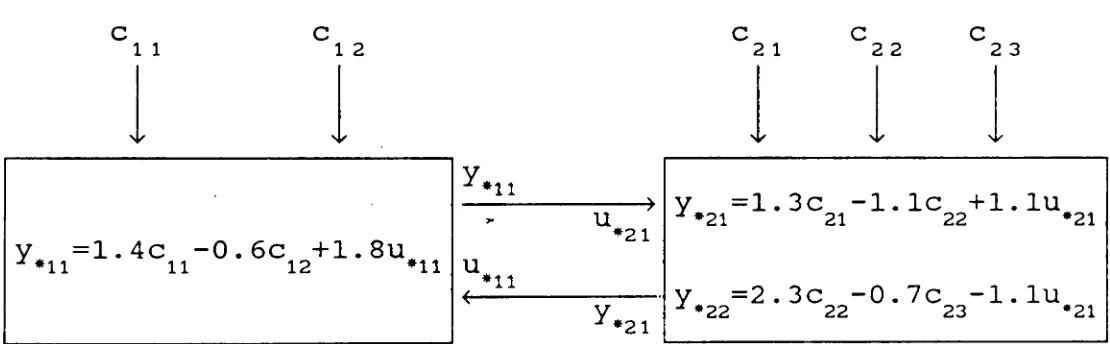
4.2 Mathematical Model of the Hierarchical Control structure

A steady state system

interconnected subprocesses,

computer, is used to

coordination methods for

model consisting of two

simulated by the analogue

investigate different

closed-loop hierarchical

control. The computer system structure used for

simulation is shown in fig.3.2.

First order time constants are introduced to the

interaction inputs and the controls. The

mathematical model of the subprocess output equations

.

Yll f ₁₁ (S:1 ' ~1) C 11

-

Y21 - f 21 (c , u ) -2 -2

-

-

Y22 f 22 (c , -2 ~) 2c 22

-

-

The performance indices are:

Q (c , u , v ) - (Y11-1)2 + C

1 2

1 + C12 2 1 -1 -1 "1

The reality output equations are:

f (c u) 1.4c - O.6e + 1.8u

I

Y *11 :lt11 -1'-1 11 12 *11

f (c u) - 1.3e - 1.le + 1.lu

Y.21 *21 -2'-2 21 22 -21

f (e

u)

-

-

1.lu

J

The system constraints are:

The coupling equation is :

U 11

U

21

y ~o, (0. 8-c -0. 6u )~O}

11 12 11

o

o

1 o

o

1

The mathematical model of the interconnected sub~rocesses

trikpn from Robr-'.rts P.D. (1982).

4.3 Summary

Mathematical

problem using

formulation of large scale control

system approach was

the hierarchical

presented in this chapter. The original control

problem, with a pre-defined overall performance index

and system constraints, was decomposed into a collection

of smaller scale subproblems. Then, the model of each

subproblem was formulated with the task to optimise its

performance index subj ected to the constraints imposed.

Once all the subproblems were formulated, the global

control problem can then be formed by assuming that the

overall performance index

indices of the subproblems.

system model consisting

subprocesses, simulated by

included.

was the sum of performance

Finally, the steady state

of two interconnected

an analogue computer, was

41

CHAPTER 5 _{ON-LINE COORDINATION METHODS}

5.1 Introduction

Different coordination methods have been suggested and

developed in the last two decades for steady state

optimisation and control of large scale systems (Mesarovic,

1970; Findeisen, 1978). Basically, there are two principal

coordination methods, namely, the Interaction Prediction Method (IPM) and Interaction Balance Method (IBM). These

coordination methods are similar in the sense that they start the local decision optimisation problem in the lower

level by specifying intervention parameters from the

supremal level. The method by which the supremal level

calculates the coordination parameters and intervenes the infimal level defines the coordination strategy. A variety

of feedback schemes have been suggested for on-line

optimising control using these coordination methods.

Feedback informations from the simulated real process used

by the coordinator (global feedback) or local decision

units (local feedba~k) have been

distributed hierarchical computer

implemented

system to

uSlng study

the

the

on-line coordination method the interaction balance

coordination

strategy.

and interaction prediction coordination

section 5.2 describes the closed-loop coordination

methods. Examination of these methods for on-line

closed-loop control of simulated interconnected industrial

processes has been performed and difficulties encountered

during the investigation will be discussed ln the

subsequent sections.

5.2 Closed-loop Coordination Methods

Using open-loop implementation of coordination methods