Control of solar sail periodic orbits in the elliptic three-body problem

Control of Solar Sail Periodic orbits in the Elliptic

Three-Body Problem

James D. Biggs

_{Colin R. McInnes}

_{Thomas Waters}

1.

Introduction

A Solar sail consists essentially of a large mirror, which uses the momentum change due to photons

reflecting off the sail for its impulse. Solar sails are therefore unique spacecraft as they do not require fuel

for propulsion.1 _{In this note we consider using the solar sail to continuously maintain a periodic orbit above}

the ecliptic plane using variations in the sail’s orientation. Positioning a spacecraft continuously above the

ecliptic would allow continuous observation and communication with the poles.

In Waters and McInnes2_{the authors identify families of periodic orbits in the solar sail Circular Restricted}

Three-Body Problem (CRTBP). In this note we model the solar sail in the context of the Elliptical Restricted

Three-Body problem (ERTBP) with the Earth and Sun as the two primaries and where the solar sail is the

third massless body. The generalization to the solar sail ERTBP is considered in Baoyin and McInnes.3 _This

highlights that a study of the elliptic case is necessary, firstly because it is a more realistic model than the

circular case and secondly because there are fundamental differences between the two cases. To begin with

there are no equilibrium points above the ecliptic in the solar sail ERTBP.3 _{Additionally, the equations of}

motion contain the time explicitly i.e. through the true anomalyf and are therefore non-autonomous. This

implies that any periodic solution of the solar sail ERTBP must have a period which is an integer multiple

of 1 year.

In this note we illustrate that a periodic orbit above the ecliptic in the circular case2 _{is not adequate for}

tracking in the solar sail ERTBP model. For this reason we illustrate two methods for obtaining “better”

periodic reference trajectories above the ecliptic for the solar sail ERTBP. The two methods we use are based

on (i) a numerical continuation, with the eccentricityeas the perturbation parameter to find a natural orbit

in the ERTBP and (ii) a time-delayed feedback mechanism, which can be used when a differential corrector

fails to converge.

∗_{, [email protected], Research Fellow, Department of Mechanical Engineering, University of Strathclyde, Glasgow.}

†_{[email protected], member AIAA, Professor, University of Strathclyde, Glasgow.}

1.A. Equations of motion for the elliptic solar sail

The classical Elliptical Restricted Three-Body Problem (ERTBP) can be modeled conveniently using a

pulsating-rotating frame6 _{and in this note we follow the same convention to model the solar sail ERTBP.}3

We choose our units to set the gravitational constant, the sum of the primary masses, the Earth’s semimajor

axis about the Sun, and the magnitude of the angular velocity of the rotating frame to be unity. We shall

denote byµ= 3×10−6 _{the dimensionless mass of the smaller bodym2, the Earth, and therefore the mass} of the larger bodym1, the Sun, is given by 1−µ. Denoting byr1andr2the position of the sail w.r.t. tom1

and m2, the solar sail’s equations of motion in the rotating frame in pulsating-rotating coordinates x, y, z

are:

x′′

−2y′

=_1+e1_cosf¡_∂Ω

∂x +accx

¢

y′′

+ 2x′

= 1

1+ecosf

³

∂Ω

∂y +accy

´

z′′

+z= 1 1+ecosf

¡∂Ω

∂z +accz

¢

(1)

where (·)′

denotes differentiation with respect to the true anomalyf ande= 0.0167 is the eccentricity with

Ω =1 2(x

2_+y2_+z2_{) +}(1−µ)

kr1k +

µ

kr2k

andacc= (accx, accy, accz)T is the solar sail acceleration defined by:

acc= β(1−µ)

kr2 1k

(ˆr1·nˆ)2nˆ (2)

whereβ is the solar sail lightness number and is the ratio of the solar sail radiation pressure acceleration to

the solar gravitational acceleration, the ‘hat’ notation denotes the unit vector and ˆnis the unit normal of the

sail with respect to the Sun. We define ˆnin terms of two anglesγ andδ(radians) in the rotating-pulsating

frame:

ˆ

n= (cosγcosδ,cosγsinδ,sinγ)T ₍₃₎

While aβ value of order 0.3−0.4 is considered within the realm of possibility, to put the analysis in this

paper well within the near-term we will consider very modestβ values of order 0.05. Note that the

rotating-pulsating coordinates are related to the rotating coordinatesX, Y, Zvia the equationsX =ρx,Y =ρyand

Z=ρz, with the semi-latus rectumρ= (1−e2₎

1+ecosf. It follows that whene= 0 the equations (1) reduce to the

circular case with the rotating-pulsating coordinates equal to the rotating coordinates.

2.

Tracking the reference trajectory given in the solar sail CRTBP

In this section we use a continuous LQR controller in the solar sail ERTBP to track a periodic reference

orbit using variations in the sail’s orientation. We show that a reference orbit from the solar sail CRTBP

is not adequate for tracking in the elliptical case. To measure the quality of the reference orbit given the

maximum deflection (radians)−π/2≤ γ, δ≤ π/2 (the sail has only one reflective side) and its maximum

rate of deflection (radians per day) is −0.42 ≤γ,˙ δ˙ ≤0.42 (1 degree per hour). To begin we linearize the

equations of motion ˙X= f(X,u(t)) about the reference orbit Γ. Writing x =X−Γ and u= u(t)−ue

yields the linear system

˙

x=A(t)x+Bu (4)

where

A(t) = ∂f(X,u(t))/∂X|_X=Γ, B= ∂f(X,u(t))/∂u(t)|_u(t)=ue

From control systems theory the gain matrixK for the linear state feedback control lawu=−Kxwhich

minimizes the quadratic cost function J =

∞

R

0

xT_Qx+uT_{Rudt where Q, R are symmetric positive}

semi-definite weighting matrices and then K = R−1_BT_{P(t) where P(t) is the unique, positive semi-definite}

solution to the differential Riccati equation:

A(t)TP(t) +P(t)A(t)−P(t)BR−1_BT_{P(t) +Q= ˙P(t) (5)}

The weightsQandRare free to choose and for simplicity this freedom is reduced to one parameter by letting

Q=I6 andR=kI2, wherekis a constant. Therefore, the control effort will be penalized ifk is large and

the distance from the orbit will be penalized if k is small. The procedure for defining the time-dependent

K =Kij matrix is to numerically compute it about the reference orbit and then fit a Fourier function to

each component ofK. The simulation is run for the equivalent of 20 years real time (20 orbits). Although

this length of time is longer than the mission time for conventional spacecraft, the solar sail has the ability to

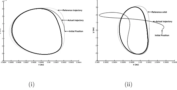
perform much longer missions. The results of this are illustrated in Figure 1. When the trajectory begins on

0.9894-4 0.98950.9896 0.98970.9898 0.9899 0.99 0.9901 0.9902 0.99030.9904 -3

-2 -1 0 1 2 3 4x 10

-3

x (au)

y

(

a

u

)

Initial Position Actual trajectory Reference trajectory

0.989 0.9892 0.9894 0.9896 0.9898 0.99 0.9902 0.9904 0.9906 0.9908 -4

-3 -2 -1 0 1 2 3 4 x 10-3

x (au)

y

(

a

u

)

Reference orbit

Initial Position Actual trajectory

(i) (ii)

Figure 1. LQR control: the thick line is the controlled trajectory and the thin dotted line is the reference orbit

(i) initial condition begins on the reference trajectory. (ii) large errors in the initial conditions are included

the reference orbit Figure 1 (i) the solar sail’s mean tracking error over 20 years is 1.5556×10−4_{au (23271} km). In Figure 1 (ii) we consider initial condition errors of approximately 25000 km with velocity errors of

tracking error is 2.1985×10−4 _{au (32889 km). These tracking errors are large and in this note we aim to} obtain “better” reference trajectories for the elliptic case.

3.

Methods to obtain reference trajectories in the Solar Sail ERTBP

In this section we propose two methods to obtain suitable periodic reference trajectories above the ecliptic

for the solar sail ERTBP. One obvious choice for a reference trajectory would be to use a natural orbit above

the ecliptic in the solar sail ERTBP. Therefore, our first method is based on a numerical continuation with

the eccentricity,e, as the continuation parameter. The second method is based on a time-delayed feedback

mechanism which is useful when a trajectories error in periodicity is too large for a differential corrector to

close it. We begin here with a description of the numerical continuation.

3.A. Numerical continuation

The continuation algorithm is based on a monodromy variant of Newton’s method.4 _{The Newton method}

starts with a trajectory X(t) = (x, y, z,x,˙ y,˙ z˙) initialized att = 0 on a surface of section and provides an

iterative improvement to the choice of initial conditions for a periodic orbit:

X∗

(0) =X(0) + (I−M)−1_{[X(T)−X(0)] (6)} where X∗

(0) is the improved initial condition and M is the monodromy matrix. We begin with a known

periodic orbit ate= 0 in the solar sail CRTBP2 _{and continue the parameterein small increments until the}

required valuee= 0.0167. The monodromy matrix required for its implementation is derived by recasting

the variational equations ((4) withu= 0) in terms of the state transition matrix (or principle fundamental

6×6 matrix) Φ = ∂X(t)/∂X(0), we have ˙Φ = A(t)Φ, Φ(0) =I. The monodromy matrix M is then

defined asM = Φ(T). Using Newton’s method we obtain initial conditions that yield a 1 year periodic orbit

above the ecliptic in the Solar Sail ERTBP:x(0) = 0.99026089327975, y(0) = 0.00000002531557, z(0) =

0.01497820748971, x′

(0) = 0.00000000062302, y′

(0) = 0.00306117310561, z′

(0) =−0.00000003900302 f(0) =

0, γ = 0.809196, δ = 0. We note that this periodic orbit is unstable and will require active control to

stabilize the solar sail on the orbit. This active control will be implemented using variations in the sail’s

orientation.

3.B. Computing reference orbits using a time-delayed feedback mechanism

In this subsection we propose a novel method for designing reference orbits based on time-delayed feedback

control.5 _{This method is particularly useful when the error in periodicity of the initial trajectory is too large}

for a differential corrector to close the orbit. To illustrate this we use a Monte Carlo simulation of initial

conditions (in a small region close to the initial conditions that yield a periodic orbit in the circular case) to

note that a differential corrector failed to close this trajectory. To compute a periodic reference trajectory

for the nonlinear system ˙X(t) =f(X(t), t) we use a time-delayed feedback mechanism of the form:

˙

X(t) =f(X(t), t) +v(t)

v(t) =−K(X(t)−X(t−τ))

(7)

whereτ is the delay time, which will be 2πin order to obtain a 1 year orbit andK is a 6×6 matrix which

is computed experimentally. By inspection of the time-delayed feedback function v(t) (7) it can be seen

that as the trajectory X(t) approaches periodic i.e. kX(t)−X(t−τ)k →0, thenv(t)→0. The nonlinear

equations (7) were simulated until the resulting trajectory satisfied the properties kX(T)−X(0)k< ε and

kv(t)k< ∂ for some pre-specified tolerance parametersεand∂.

We note that this method can be implemented using either forward integration or backwards integration

and that backward integration worked better in this case. Using the preceding method we obtained the

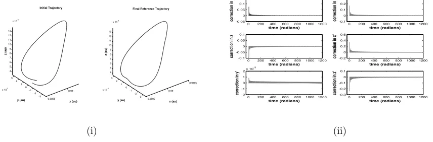
closed reference trajectory in Figure 2 (i). From Figure 2 (ii) it can be seen that the initial orbit requires

a large impulse (correction) to close the trajectory but this reduces in magnitude with time. Finally, we

0.9895 0.99 0.9905 -3 -2 -1 0 1 2 3

x 10-3

4 5 6 7 8 9 10 11 12 13 x 10-3

x (au) Initial Trajectory y (au) z (a u ) 0.9895 0.99 0.9905 -3 -2 -1 0 1 2 3

x 10-3

4 5 6 7 8 9 10 11 12 13 x 10-3

x (au) Final Reference Trajectory

y (au)

z

(a

u

)

0 200 400 600 800 10001200 -0.05 0 0.05 0.1 0.15 time (radians) co rr ec tio n in x

0 200 400 600 800 10001200 -0.1 0 0.1 0.2 0.3 time (radians) co rr ec tio n in y

0 200 400 600 800 10001200 -0.1 -0.05 0 0.05 0.1 time (radians) co rr ec tio n in z

0 200 400 600 800 10001200 -0.2 0 0.2 0.4 0.6 time (radians) co rr ec tio n in x '

0 200 400 600 800 10001200 -2

-1 0 1 2x 10

-3 time (radians) co rr ec tio n in y '

0 200 400 600 800 10001200 -0.3 -0.2 -0.1 0 0.1 time (radians) co rr ec tio n in z' (i) (ii)

Figure 2. Time-delay feedback: (i) this illustrates the initial trajectory and final closed trajectory (ii) the

corrections required to close the initial orbit is large but these decrease to small values as time increases.

test the quality of the reference orbits given by the numerical continuation and the time-delayed feedback

mechanism in simulation using the LQR method described in Section 2. The results show that there is a

vast improvement in the sail’s ability to track these reference orbits compared to the reference orbit in the

circular case. For the reference orbit computed using the time-delayed feedback method the mean tracking

error (without initial condition errors) is 1.522×10−5 _{au (2278 km). Using the same magnitude of errors} in initial conditions as the circular case, the mean tracking error is 1.9288×10−5 _{au (2885 km). For the} reference orbit found using the numerical continuation the mean tracking error (without initial condition

errors) is 4.6733×10−₈

au (7 km). This error is small as it is a natural orbit and control is required only to

4.

Conclusions

This note considers the problem of maintaining a solar sail on a periodic orbit above the ecliptic in

the Elliptical Restricted Three-Body Problem (ERTBP). We illustrate that the solar sail does not track a

periodic reference orbit obtained from the solar sail Circular Restricted Three-Body Problem adequately. We

proceed to illustrate two methods for constructing “better” reference trajectories based on (i) a numerical

continuation, with the eccentricitye as the perturbation parameter to find a natural orbit in the ERTBP.

(ii) a time-delayed feedback mechanism, which can be used when a differential corrector fails to converge.

Both these methods yield reference orbits that significantly improve the tracking error of the solar sail.

Acknowledgments

This work was funded by grant EP/D003822/1 from the UK Engineering and Physical Sciences Research

Council (EPSRC).

References

1

McInnes, C. R., ‘Solar sailing: technology, dynamics and mission applications’. Springer Praxis, pp. 17-19, 1999.

2

Waters, T. J., McInnes, C. R., ‘Periodic Orbits above the Ecliptic in the Solar sail Restricted Three-body problem’. Journal

of Guidance, Control and Dynamics, Vol. 127, pp. 1947-1960, 2007.

3

Baoyin, H., McInnes, C.R., ‘Solar sail equilibria in the elliptical restricted three-body problem’. Journal of Guidance,

Control and Dynamics, Vol. 29, No. 3, pp. 538-543, 2006.

4

Marcinek, R., Pollak, E., ‘Numerical methods for locating stable periodic orbits embedded in a largely chaotic system’.

Journal of Chemical Physics, 100, 8, pp. 5894-5904, 1994.

5

Pyragus, K., ‘Continuous control of chaos by self-controlling feedback’. Physics Letters A, Vol. 170, pp. 421-428, 1992.

6

Szebehely, V., ‘Theory of Orbits: The restricted problem of three bodies’. Academic Press, New York, pp. 587-595, 1967.