A Search for MRI diffusion coefficient standards

Rochester Institute of Technology

RIT Scholar Works

Theses Thesis/Dissertation Collections

10-1-2011

A Search for MRI diffusion coefficient standards

Hongmei Yuan

Follow this and additional works at:http://scholarworks.rit.edu/theses

This Dissertation is brought to you for free and open access by the Thesis/Dissertation Collections at RIT Scholar Works. It has been accepted for inclusion in Theses by an authorized administrator of RIT Scholar Works. For more information, please [email protected]. Recommended Citation

A Search for MRI Diffusion Coefficient Standards

Hongmei Yuan

M.S. Physical Chemistry, Wuhan University, Wuhan, P.R.China, 2004 B.S. Chemical Education, Xinyang Normal University, Xinyang, P.R.China, 2001

A dissertation submitted in partial fulfillment of the

requirements for the degree of Master of Science in the

Department of Chemistry,

College of Science

Rochester Institute of Technology

October 2011

Signature of the Author _________________________________

DEPARTMENT OF CHEMISTRY COLLEGE OF SCIENCE

ROCHESTER INSTITUTE OF TECHNOLOGY ROCHESTER, NEW YORK

CERTIFICATE OF APPROVAL

________________________________________________________________________

M.S. DEGREE DISSERTATION

________________________________________________________________________

The M.S. Degree Dissertation of Hongmei Yuan has been examined and approved by the dissertation committee as satisfactory for the dissertation required for

the M.S. degree in Chemistry.

____________________________________________ Dr. Joseph Hornak, Dissertation Advisor

____________________________________________ Dr. Christopher Collison

____________________________________________ Dr. Lea Michel

____________________________________________ Dr. Thomas Smith

____________________________________________ Date

i Abstract

Diffusion coefficients (D) can be readily measured by nuclear magnetic resonance

(NMR) spectroscopy and magnetic resonance imaging (MRI) instruments. Operators of

these instruments often utilize standards with known diffusion coefficients to rapidly and

conveniently test the performance of the NMR or MRI system to measure diffusion. A

variety of these standards have been proposed in the scientific literature. This thesis

describes a diffusion standard based on water constrained by container geometry,

specifically water between tightly packed, parallel glass fiber filaments. The restricted

diffusion of water in this environment gives a diffusion coefficient which is selectable by

the choice of data acquisition parameters. Thus, one standard can be used to achieve

multiple diffusion coefficients and replaces the need for multiple diffusion standards.

Educational training was performed on a 300 MHz NMR spectrometer located at

Rochester Institute of Technology (RIT). As a part of this training, pulsed magnetic field

gradient strengths were calibrated and diffusion coefficients (D) measured for a series of

silicone oils of different viscosities.

Diffusion coefficient values for a small diameter test phantom were measured on a

600 MHz NMR spectrometer with stimulated echo pulse sequence at 25°C. A

predictable behavior between the apparent diffusion coefficient and gradient separation

() value in the sequence was observed. Diffusion coefficient values were measured for

a larger diameter phantom using a 1.5 T imager at 20°C using echo-planar imaging

sequence and confirmed to follow the same D vs.  behavior. Based on these

observations, a hydrated fiber bundle can make a diffusion phantom with only water

ii

ACKNOWLEDGEMENT

My deepest thanks to Dr. Joseph Hornak, my research advisor. This thesis would

not have been possible without Dr. Hornak’s great assistance and encouragement. Thanks

also to Dr. Hornak’s wife, Elizabeth Hornak, whose enthusiasm and kindness makes me

feel like a part of an American family. Thanks to my other thesis committee members, Dr.

Thomas Smith, Dr. Christopher Collison, Dr. Andreas Langner, and Dr. Lea Michel, for

their assistance and encouragement during my studies at Rochester Institute of

Technology. I am especially thankful to Dr. Paul Rosenberg, Brenda Mastrangelo, and

Autumn Madden for their care and attention, as well to the RIT Chemistry Department

for supporting me.

I also wish to thank Dr. Scott Kennedy at the University of Rochester Biophysics &

Biochemistry, Dr. Edmund Kwok from the Imaging Science Department at the

University of Rochester Medical Center, Dr. Paul Keifer at Varian Inc., and Dr. Amy

Freund at Bruker Biospin Inc., who have supported instruments and measurements in this

work.

Special thanks should be given to my ESL teachers, Lisa Hoffmaster and Linda

Gamlen, to my student colleagues, Can Wang, Yuqiong Joan Wang, Yujie Qiu and her

husband, Wei Yao, Jennifer Swartzenberg, and Luticha A. Doucette, who helped me in

many ways in America. Finally, words alone cannot express the thanks I owe to my

family members in China and Shunxu Ge, my husband for their encouragement and

iii

Table of Contents

Abstract……….i

Acknowledgements………..ii

1.0 Introduction………1

2.0 Background and Theory……….4

2.1 Diffusion………...4

2.2 Nuclear Magnetic Resonance………...9

2.3 Pulse Sequences………..12

2.4 Magnetic Resonance Imaging……….20

3.0 Experimental Methods……….23

3.1 Sample Preparation……….23

3.2 NMR Spectroscopy……….25

3.3 Gradient Calibration………26

3.4 MRI Measurements……….28

4.0 Results and Discussion…...29

4.1 Gradient Calibration Results………...29

4.2 Diffusion Coefficient Checks……… 31

4.3 Diffusion Coefficient from the 600 MHz NMR……… 34

4.4 Diffusion Coefficient from the 1.5T MRI System………..35

5.0 Conclusion………...39

1

1.0 Introduction

In the last three decades, magnetic resonance imaging (MRI) has established itself

as the most diagnostically useful imaging modality in the medical imaging field. It is in

part because of the ability of MRI to distinguish between soft tissues in the body. The

last decade has seen the emergence of a new kind of MRI, quantitative MRI.

Quantitative MRI uses MRI to measure some specific property, such as the diffusion

coefficient, and relate it specifically to a disease state.

Some studies have related the diffusion coefficient of water in tissues to a disease

state such as ischemia [1-4], epilepsy [5-7], tumors [8-10], and strokes [11-13]. Magnetic

resonance imaging is capable of producing several forms of images yielding diffusion

information. These include diffusion weighted, diffusion, and diffusion tensor images.

Diffusion weighted images are magnetic resonance images where contrast is related to

the diffusion coefficient. Diffusion imaging produces images of the diffusion coefficient.

Diffusion tensor imaging (DTI) produces images of the diffusion tensor of water in each

location in the image. The technique has been especially useful in mapping the tracks of

nerve fibers in the brain, and therefore determining interconnectivity in the brain.

Quantitative magnetic resonance imaging studies of diffusion require a standard, or

phantom, to calibrate the imaging system. A phantom is an anthropogenic object used to

test the performance of the imaging system. The term phantom is more commonly used

by the MRI community. Several diffusion phantoms have been proposed in the literature.

These include liquids with an isotropic D value [14-17], plants [18-20], biological

2

Phantoms utilizing isotropic liquid consists of a set of hydrocarbon liquids with self

diffusion coefficients (D) between that of water and approximately 0.5x10-9 m2/s. [17]

Shipping constraints make commercializing phantoms containing flammable

hydrocarbons more costly. Plants and biological based phantoms are difficult to keep for

long periods of time as they degrade and the diffusion coefficient changes. Capillary

phantoms have a low signal, because a large amount of the phantom volume is the

capillary tube compared to the smaller amount of signal bearing liquid, which causes

large susceptibility artifacts in the images.

Phantoms based on fibers overcome many of the previously mentioned

shortcomings and have some notable advantages, namely the ability to calibrate and

characterize DTI. Several fiber phantoms have been reported recently [28-29] for

quantitative studies. Lorenz, et al. [28] reached the conclusion that the hydrophobic

fiber materials polyamide and Dyneema® (an ultra-high molecular weight polyethylene

[30]), showed greater anisotropy, as well as much higher alignment along the actual fiber

direction than the hydrophilic fiber materials hemp, linen, and viscose rayon. Fieremans,

et al. [29], introduced a fiber phantom made of ultrahigh-molecular-weight polyethylene

(micro dyneema). This kind of fiber phantom was proved to be suitable for the

quantitative validation of diffusion imaging because of the correspondence between the

simulations and the experimental results. The result of their three-dimensional Monte

Carlo simulation of random walker demonstrated that the diffusivity for the random

packing geometries with a fixed diameter was similar to the diffusivity for a random

3

there is intracellular and extracellular diffusion [31], but currently, fiber materials with

such exact diffusion properties are not available.

This thesis proposes a diffusion phantom based on the restricted diffusion of water

between tightly packed glass fibers. This form of phantom has been developed for

diffusion tensor imaging [28-29, 32-35], but not as a solution to the stated problem. This

phantom should yield a range of diffusion coefficients less than Dwater as a consequence

of restricted diffusion using only water as the nuclear magnetic resonance signal bearing

liquid. As a consequence, shipping of the phantom should be easier.

This thesis describes a project designed to test the hypothesis that a phantom based

on restricted diffusion can be used as a calibration standard for MRI. There are two parts

to the test. Restricted diffusion samples will be designed, prepared and tested on a

high-resolution NMR spectrometer capable of measuring diffusion coefficients. Once a

standard is developed on this system, it will be scaled up in size and tested on a clinical

system. I planned to use the Bruker DRX 300 MHz NMR spectrometer located in the

RIT Chemistry Department for the first phase of the project. The calibration of the

system was completed but, unfortunately, a series of maintenance problems with the

spectrometer forced us to look elsewhere for these measurements. Therefore all tests on

high resolution systems were performed on a 600 MHz system located at the University

of Rochester. The calibration results were included in this thesis to explain the process,

but the University of Rochester performed their own gradient calibration procedure. MRI

4

2.0 Background and Theory

2.1 Diffusion

Diffusion is the random movement of molecules or particles due to the kinetic

energy of the molecules and particles. This definition is broad and covers a great deal of

science. To help the reader see the connection of this research to the field of diffusion, a

broad overview of diffusion will be presented first, followed by a focus on aspects more

specific to this research.

The introductory student of diffusion will encounter several terms that should be

described first. These include self, mutual, counter, free, restricted, anisotropic, isotropic,

translational, and rotational diffusion; in addition to the true and apparent diffusion

coefficients. Self-diffusion is the motion of a particle when the concentration gradient is

zero. This motion is what we are familiar with when we say Brownian motion. Mutual

or Counter diffusion is the motion of a particle in the presence of a concentration (C)

gradient. Mutual or Counter diffusion is described by Fick’s laws [36] of diffusion.

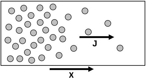
Fick’s first law of diffusion describes the diffusion of particles from a region of

high concentration to a region of low concentration. (See Fig. 2.1.) The flux (J) in the x

direction is a result of a concentration gradient (C/x). The flux goes from regions of

high concentration to regions of low concentration. J is proportional to C/x by a

constant called the diffusion coefficient (D) for the diffusing particles.

J = -D (C/x) (2.1)

Fick's second law of diffusion describes the change of concentration with respect to

time (t).

5

For spherical particles of radius r, the self diffusion coefficient in absence of a

concentration gradient at temperature T is directly related to the viscosity (η) of a

material through the Stokes-Einstein equation [37],

r 6

T k

D B

 

 (2.3)

where kB is the Boltzmann constant. The diffusion coefficient is temperature dependent

and increases with increasing temperature. The diffusion coefficient in the international

system (SI) of units has units of m2/s. The self diffusion coefficient of water at 25 °C is

2.299×10-9 m2/s [38].

Diffusion can be classified as restricted and unrestricted. Unrestricted diffusion is

what occurs in outer space where there are no boundaries. Because most physical

experiments are performed on Earth and are constrained by boundaries of one form or

another, there is restricted diffusion. In practice, we can talk about both unrestricted and

restricted diffusion on Earth. Unrestricted or free diffusion is the diffusion unlimited by

J

X

6

the size of the container, while restricted diffusion is the diffusion limited by the size of

the container. Diffusion can be restricted in one, two, or three spatial dimensions.

It is possible in ordered media to have diffusion vary with direction. Examples of

ordered media include nematic, smectic, cholesteric, columnar phases of liquid crystals;

water bound on a surface; and mono- and bi-layers of surfactant-like molecules. It is also

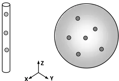
possible to have diffusion vary with the shape of a container. Figure 2.2 shows examples

of restricted and less restricted diffusion due to the shape of the container. Diffusion of

particles in a narrow cylinder with long axis along Z may experience unrestricted

diffusion in Z but restricted diffusion in X and Y. The diffusion of particles within a

large sphere will experience less restricted diffusion, especially on a short time scale.

This introduces the need to think of the diffusion timescale. In the case of any shaped

container, diffusion is unrestricted if the particles do not encounter the wall of the

container during the time of a measurement. If they do encounter a wall there is

restricted diffusion. The root-mean-squared distance traveled by a particle in time t is

given by Eqn. 2.4, where qi is a dimensionality constant which accounts for the

dimensionality of the container [37]. The constant takes on values of 2, 4, and 6 for

respectively 1, 2, and 3 dimensions.

<x>2 = qi D t (2.4)

It is worth mentioning at this point that the material composition of a container can

have an effect on the liquid within it. For example, a polar solvent such as water in a

hyrdophylic container will form a layer of bound water on the surface. This surface layer

of water has very different properties than bulk or free water far from the surface. The

7

larger in diameter, this bound layer is insignificant compared to the total volume of water.

At micrometer diameter dimensions and smaller, the volume of this layer becomes

significant. Therefore, water in small capillary tubes and between the fibers of a tightly

packed set of fibers will exist in two forms: bulk and bound. The bound water will

possess a diffusion coefficient different than bulk water. Measurements of water in these

environments can yield two values: a small D value for the bound water and a larger one

for the bulk water.

Diffusion, which is the same in all dimensions, is called isotropic, while anisotropic

diffusion is not the same in all directions. For anisotropic diffusion, D is not the same in

all directions, while for isotropic diffusion, D is independent of direction. A diffusion

tensor can be used to describe anisotropic diffusion.

A tensor is an abstract object used to express a multi-dimensional concept. It can be

used to represent the diffusion coefficient in three dimensions or six directions. The

Z

X Y

Figure 2.2 A depiction of restricted and unrestricted diffusion in a narrow cylinder and a large sphere. In the cylinder, diffusion is restricted in X and Y while unrestricted in Z. In

8

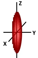
following three-dimensional tensor expresses the diffusion in a narrow cylinder as

depicted in Fig. 2.3.

Thus far, the presentation of diffusion has been restricted to translational diffusion

or the motion of the particles as a whole unit. Although not the subject of this thesis, it is

possible to discuss rotational diffusion. Rotational diffusion is the motion of part of a

molecule rotating around a bond. An example of this is the rotation of methyl hydrogens

when the methyl group rotates about the carbon bond. (See Figure 2.4.)

Scientists often distinguish between two diffusion coefficients: the true diffusion

coefficient (TDC) and apparent diffusion coefficient (ADC). The TDC is the diffusion

coefficient for free diffusion, while the ADC is the measured diffusion coefficient. For

restricted diffusion, the ADC is less than the TDC because the size of the container limits

the diffusion distance.

C H

H H

Figure 2.4 A schematic representation of rotational diffusion of the hydrogen atoms on a methyl group about a carbon bond.

Z

X

Y

9 2.2 Nuclear Magnetic Resonance

Electrons, protons, and neutrons possess a fundamental, quantum mechanical

property of matter called spin. The spin of each of these particles can take on values of

+½ and –½ [38]. The property spin can be thought of as a magnetic moment possessed by

the particle. The spin of particles in close proximity can combine to give a net spin and

magnetic moment of zero or some higher value. For example, a molecule or atom with

two unpaired electrons in a triplet configuration will have possible spin values of +1 , 0,

and –1. A nucleus with a single unpaired proton, such as hydrogen, will have values of

+½ and –½, while the nucleus of sodium-23 with one unpaired proton and two unpaired

neutrons can have spin values of 3/2, 1/2, -1/2, and -3/2.

When placed in a magnetic field, matter with a non-zero spin can absorb

characteristic energies due to a splitting of the energy states of the spins [39-41]. Two

spectroscopies focus on this absorption of energy. Electron spin resonance (ESR)

spectroscopy focuses on matter with electron spin, while nuclear magnetic resonance

(NMR) spectroscopy focuses on matter with nuclear spin. This thesis focuses on the use

of NMR spectroscopy to measure diffusion, so the remaining theory will focus on NMR.

For a simple spin ½ nucleus, such as a hydrogen-1 nucleus, the spin has two energy

levels when placed in a magnetic field (Bo). The energy difference (E) between these

two levels is given by

E = h (2.5)

where h is Planck’s constant, and is the frequency of a photon. The value of can be

10

=Bo (2.6)

where  is a proportionality constant called the gyromagnetic ratio for the nucleus. For

hydrogen, = 42.58 MHz / T [39-41]. In the classical picture of magnetic resonance,  is

the rate at which a particle with spin precesses about the direction of the applied magnetic

field.

The relative populations of the two levels (N+ and N-) at temperature T is given by

Boltzmann statistics where k is Boltzmann’s constant.

N-/N+ = e-E/kT (2.7)

The net magnetization (M) from a group of spins is proportional to (N+ - N-). It is the

value of M that is probed in NMR spectroscopy. At equilibrium, the net magnetization

takes on a value Mo. The NMR experiment can perturb the value of M making it other

than the value Mo. Following the return of M to Mo can provide useful information about

a physical system.

If the population difference of the two spin states is not at equilibrium, the

distribution wants to return to equilibrium. The driving force returning the spins to

equilibrium is random molecular motions at  and 2 which produce time varying

magnetic fields (photons) which cause transitions between the energy levels and hence

reestablish equilibrium. This process is called spin-lattice relaxation [39]. Spin-lattice

relaxation is a first order kinetic process which is governed by a first-order time constant

called the spin-lattice relaxation time (T1).

Since particles with spin are said to precess about the direction of an applied

11

perpendicular to the direction of Bo. This transverse magnetization does not exist at

equilibrium as there is no phase coherence of the precessional motion. If a transverse

component of magnetization is established in a sample, it will eventually be lost due to

spin exchange between nuclei and due to the spins existing in an inhomogeneous applied

magnetic field. The loss of transverse magnetization is referred to a spin-spin relaxation.

Spin-spin relaxation is characterized by a first order decay time constant called the

spin-spin relaxation time. Magnetic resonance scientists distinguish between spin-spin-spin-spin

relaxation processes caused by the intramolecular spin exchange (T2) and those caused by

an inhomogeneous magnetic field (T2Inhomo). The combined spin-spin relaxation is

referred to as T2 star (T2*) [39]

1/T2* = 1/T2 + 1/T2Inhomo (2.8)

A spin system can be caused to have an MMo and a transverse magnetization by

the application of an oscillating magnetic field (B1) (again photons) at . In magnetic

resonance we adopt a Cartesian coordinate system to describe this process. In this

example, B is applied along +Z and M can have an X, Y, and Z component. The system

of coupled differential equations which describe the classical behavior with respect to

time of magnetization from a spin system are called the Bloch equations. For simplicity,

the Bloch equations [39] are often presented for a frame of reference rotating at  about

Z. This rotating frame is referred to as the (X’,Y’,Z) frame of reference.

dMX’/dt = 2(oMY’ – MX’/T2 (2.9)

dMY’/dt = – 2(oMX’ +2B1MZ –MY’/T2 (2.10)

12

The Bloch equations can be solved to show the behavior of magnetization after or

during any perturbation. For example, the application of a B1 field along X’ for a period

of time  will rotate M about X’ by .

 = 2 B1 (2.12)

If M is rotated from its equilibrium position along +Z to +Y’ by what is called a 90o

B1

pulse along X’, Mz will return to Mo according to

MZ = Mo(1-e-t/T1). (2.13)

Transverse Y’ magnetization at o behaves according to

MY’ = Mo e-t/T2 , (2.14)

while MX’ = 0 under these conditions. When   o, transverse magnetization precesses

about Z at frequency (-o) and exponentially decreases to zero.

MX’ = -Sin(2(-o)t) e-t/T2 (2.15)

MY’ = Cos(2(-o)t) e-t/T2 (2.16)

2.3 Pulse Sequences

Equations (2.13) through (2.16) form the basis of a simple magnetic resonance

experiment and signal. Magnetization is perturbed from equilibrium and evolves back

toward equilibrium. The evolution towards equilibrium causes time varying magnetic

fields in the sample which can induce a current in a coil of wire placed in a transverse

place and adjacent to the sample. The signal generated by My’ and Mx’ is called a free

induction decay (FID) [37, 39]. The FID decays exponentially with time constant T2*

13

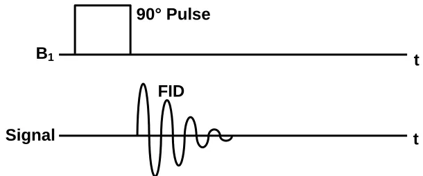
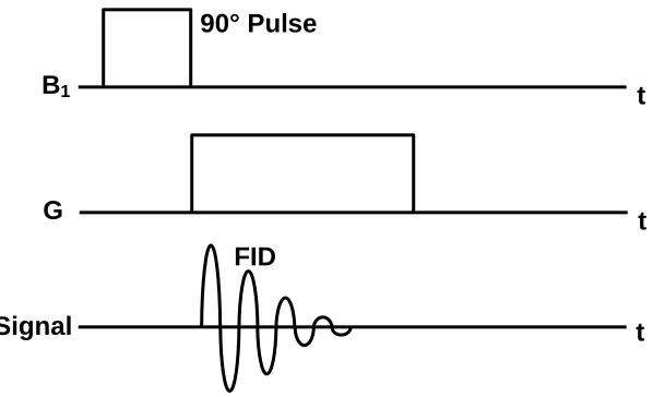
The previous example described a simple 90°-FID pulse sequence. (See Fig. 2.4.)

A pulse sequence is the application of one or more B1 pulses which generate a signal

from the sample. There are numerous pulse sequences. The 90°-FID pulse sequence

applies a 90° B1 pulses which creates an FID. The FID is a time domain signal which can

be Fourier transformed to produce a frequency domain representation of the frequencies

in the sample.

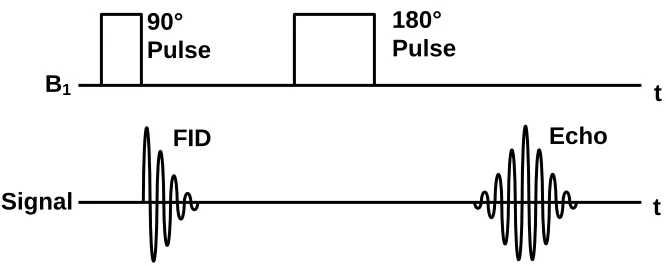
Another common pulse sequence is the spin-echo pulse sequence. (See Fig. 2.6.)

The spin-echo sequence consists of two B1 pulses, one 90° and one 180° pulse. The 90°

pulse rotates magnetization into the XY-plane where it dephases according to T2*. The

180° pulse refocuses the magnetization and creates a signal called an echo. The echo

grows and decays exponentially according to T2* [39, 41]. The echo amplitude (S)

decays from its maximum value (So) when the time between the 90° pulse and the 180°

pulse (TE) is zero.

2 E/T

T o e

S

S  (2.17)

Figure 2.5 A timing diagram for a 90°-FID pulse sequence.

t

t B1

Signal

90° Pulse

14

The spin-echo sequence is special because it allows the separation of spin-lattice

relaxation processes from molecular interactions and spin-lattice relaxation processes

from inhomogeneities in the magnetic field. The echo grows and decays according to T2*

while the echo amplitude decays exponentially with respect to TE with T2.

One additional aspect of the spin-echo sequence is worth noting because of its

relevance to diffusion. Assuming spins are located in an inhomogeneous magnetic field,

the signal from moving spins does not completely refocus at TE, while the magnetization

from stationary spins will. This forms the basis of the pulsed magnetic field gradient

diffusion measuring techniques.

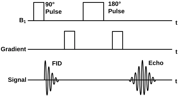
Consider the spin-echo pulse sequence of Fig. 2.7. It differs from that of Fig. 2.6 by

the addition of two periods of time when a linear one dimensional gradient in the Bo

magnetic field is turned on. The gradients in the Bo field are momentarily applied. The

first gradient pulse causes spins at different locations in the gradient direction to precess

at different rates according to their position in the gradient direction. The second

gradient pulse allows reversal of any dephasing that occurred due to the first pulse when

Figure 2.6. A timing diagram of the spin-echo pulse sequence

t

t B1

Signal

90° Pulse

FID

180° Pulse

15

the spins are stationary. Spins that move to a new location between the first and second

gradient pulse are not refocused, and diminish the amplitude of the echo. Therefore, the

echo amplitude becomes a function of the diffusion coefficient of the spins. This pulse

sequence is referred to as a pulsed field gradient spin echo (PGSE) sequence [37, 39, 41].

The signal (S) in the presence of the gradient (GDiff) compared to the signal in the

absence of the gradient (So) is given by Eqn. 2.18 [41]

bD

o

e S

S _

 (2.18)

where                 6 30 3 ) 2 ( 2 3 2 2

2    

  G_Diff

b . (2.19)

The gradient pulse quantities , , and ζ refer to pulse separation, width, and risetime

respectively, as defined in Fig. 2.8.

Figure 2.7. A timing diagram of the pulsed field gradient, spin-echo pulse sequence

t B1 90° Pulse 180° Pulse t Signal

FID Echo

16

The diffusion gradient must be one-dimensional (1D), linear, and well characterized. D

is often determined.

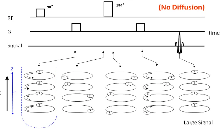
A detailed scientific description of the PGSE sequence can be very lengthy without

analogies. The race track analogy will be used to describe the effect of the PGSE

sequence on a spin system. The reader is instructed to refer to Fig. 2.9 while reading this

description. Figure 2.9 presents the timing diagram and pictures of a subset of four spins

in the NMR sample tube. The precessional frequency and phase of the magnetization

from the set of spins is depicted as runners on a race tract. The gradients in the PGSE

sequence are applied along the Z direction in this depiction such that the magnetic field at

any point along Z is (Bo + ZGz). The speeds of the spins in this description are relative to

the rotating frame frequency implying that spins experiencing Bo at Z=0 do not precess.

For this presentation the spin-spin and spin-lattice relaxation times are assumed to be

infinite.

If there is no diffusion between the application of the 90° RF pulse and the first

gradient pulse, spin #1 goes around the track with the fastest speed because the gradient

pulse speeds up the spin. The spin #4 goes fast in the opposite direction because of a

reverse magnetic field contribution from the gradient. Spins #2 and #3 go around the



G

t





G

17

track at slower speeds in opposite directions. Each spin acquires a phase which is

proportional to its position Z. The spins reverse direction after the 180º pulse. Because

they experience the same magnetic field the gradient pulse before and after the 180º pulse,

the spins come back to their starting position at the peak of the echo. In reality, the spins

will not come back into phase completely due to spin-spin relaxation. The configuration

of all spins being aligned gives a large signal.

If diffusion occurs during the pulse sequence, the movement of the spins on the

racetrack looks different. (See Fig. 2.9b.) After the 90° RF pulse and during the first

gradient pulse, the spins rotate with the same speed and the same directions as they did in

Fig. 2.9a. Now we assume they can move randomly among the different tracks. Before

the 180° RF pulse the four spins are in different tracks. There is nothing specific about

the order presented in the figure, the important point is they are randomized. The 180°

pulse does the same thing as in Fig. 2.9a, it flips the four spins to the other side. The

gradient pulse is turned on again and spins move at specific rates around the tracks

depending on their position. Because of diffusion the spins can end up on different tracks

and they do not come back to the starting line in phase. We now see less signal than the

case without diffusion. In reality the spins are constantly diffusion. The lost signal is

related to the diffusion coefficient, the gradient strength, gradient length, and gradient

18

Fig. 2.9a. The race track analogy for a PGSE sequence in the absence of diffusion.

19

There are several variants on the PGSE pulse sequence. These variations were

developed to compensate for eddy currents in the NMR system. Eddy currents are

electrical currents induced in a conducting surface when exposed to a changing magnetic

field. These eddy currents create their own magnetic field which distorts the desired

magnetic field.

Measurements of D as a function of  with constant  show the effects of restricted

diffusion when   xc2 /qiD. Under these conditions, the measured diffusion coefficient

is less than the actual diffusion coefficient for the liquid in an unrestricted environment.

We have capitalized on restricted diffusion to create a phantom that will give selectable D

values through the choice of  value and phantom orientation. An added feature of the

phantom is that D is anisotropic, also allowing calibration of diffusion tensor imaging

sequences. The concept is first demonstrated on small samples using the flexibility found

on a high-resolution NMR spectrometer, then scaled up in size to produce a phantom for

a clinical instrument.

Figure 2.10 A timing diagram of the pulsed field gradient stimulated echo sequence.

t GDiff

t B1

90° 90° 90°

180° 180°

20 2.4 Magnetic Resonance Imaging

The basis of all MRI is Eqn 2.6 which states that the resonance frequency is

proportional to the magnetic field experienced by the nuclear spin [37, 39]. If a

one-dimensional, linear, magnetic field gradient Gi is applied along direction di, Eqn. 2.6

becomes

=Bo + diGi) (2.20)

Thus the frequency becomes dependent on the location of a spin. Fourier based

tomographic imaging sequences generally apply a slice selection (S) gradient followed by

phase () and frequency (f) encoding gradients to produce N×Nf pixel images of the

NMR signal in a slice of thickness (Thk) through an object. The field-of-view (FOV)

refers to the width of the image in distance units. All gradients and frequencies are

measured relative to a point referred to as the magnet isocenter where the distances in the

slice, phase, and frequency encoding directions, respectively dS, d, and df, equal zero and

the resonance frequency is o.

A simple 1D imaging sequence can be implemented by applying a 90º B1 pulse

followed by the application of a magnetic field gradient. (See Fig. 2.11.) This sequence

21

There are many imaging pulse sequences [41]. The echo-planar imaging sequence

will be presented because it was used in this work. The echo-planar sequence is similar

to a spin-echo sequence in that there are 90º and 180º B1 pulses of radio frequency (RF).

(See Fig. 2.12.) Positioning of a tomographic slice is achieved by the application of B1

pulses at the same time a slice selection gradient Gs is applied. Phase and frequency

encoding is achieved by the application of gradients, G and Gf respectively,

perpendicular to Gs. The signals produced by each reversal of Gf create the lines of

k-space which correspond to the image. This data is Fourier transformed to create the

image.

Figure 2.11 A timing diagram for a simple one-dimensional imaging sequence utilizing a 90°-FID pulse sequence.

t B1

90° Pulse

t Signal

FID

22

The echo-planar imaging sequence can be utilized to create diffusion images by

adding the GDiff pulses of Fig. 2.8. These pulses are centered about the 180º pulse so that

the last GDiff pulse is completed before the succession of G and Gf pulses. The signal in

the form of an image created with GDiff (S) is compared with that in the absence of GDiff

(So) using Eqn. 2.18 to obtain D. GDiff can coincide with GS, G or Gf, thus D can be

calculated along any direction.

23

3.0 Experimental Methods

3.1 Sample Preparation

Several samples of poly(dimethylsiloxane) (Sigma-Aldrich, St. Louis, MO, USA),

referred to as silicone oil, were used to gain experience measuring diffusion coefficients

on an NMR spectrometer. These samples ranged in average molecular weight yielding

viscosities of 5, 10, 20, 50, 100, 350, and 500 cSt.

Several samples of 18 M∙cm water in various restricted diffusion geometries were

studied. NMR sample geometries included a 1 mm ID capillary tube and a 3 mm

diameter hand-made bundle of 11 ± 2 m diameter, approximately parallel, glass fiber

rods held together with 0.42 cm OD shrunken heat-shrink tubing. Both samples were

centered in 5 mm OD NMR tubes. The 1mm tube was filled with water, while the fiber

bundle was hydrated by allowing water to be drawn up into the fibers. If fibers of

diameter d are perfectly aligned and hexagonally packed, the fiber bundle creates long

channels between the fibers with a maximum diffusion distance perpendicular to the long

axis of the fibers of 0.732d, With this packing geometry, the water percent in the bundle

is approximately 9%. Assuming a less efficient, square packing, the maximum diffusion

distance perpendicular to the long axis of the fibers is d and there is 20% water in the

bundle. Our packing is probably a mixture of the two packing geometries.

Anoptical microscope with digital camera (Eclipse E600PL, Nikon, Tokyo, Japan)

and image analysis software (analySIS, Olympus Soft Imaging System GmbH, Berlin,

Germany) was used to determine the diameters of the fibers in the samples.

The MRI sample geometry consisted of a 2.8 cm diameter, 9.5 cm long, hand-made

24

shrink tubing. The bundle was hydrated by allowing water to be drawn up into the

bundle and then it was supported in a water filled container.

The manufacturing flow chart of the 3mm diameter hand-made fiber phantom for

NMR measurements is shown in Fig. 3.1. First, a bundle of parallel fibers is pulled

through a piece of heat-shrinkable tubing. The tubing is shrunk to hold the fibers tightly

together. This is depicted for larger fiber rods in Fig 3.1a. Second, one end of the

hand-made bundle is glued together. The shrink tubing is removed once the glue is set. (See

Fig. 3.1b.) The next step is to insert the bundle into an NMR tube. Once inserted, 18

M∙cm water is allowed to absorb into the fibers. An ultrasonic bath and vacuum are

used to remove any bubble inside of the NMR tube. The diffusion is of the water

between solid fiber filaments.

A scaled-up glass fiber phantom with diameter of 2.8 cm was hand-made in the

similar way as that of the fiber phantom for the NMR measurements. It is used for the

MRI measurements. See Fig. 3.2.

a b c

25 3.2 NMR Spectroscopy

NMR measurements were performed on two different NMR spectrometers. Initial

measurements were performed on a 300 MHz NMR spectrometer (DRX-300, Bruker

Biospin, Billerica, MA, USA) with three axis gradients located at Rochester Institute of

Technology (RIT). This system became inoperable after these initial measurements

requiring measurements to be made on an alternative system.

A 600 MHz NMR spectrometer (UnityInova, Agilent-Varian Inc., Walnut Creek,

CA, USA) with three axis gradients located at the University of Rochester was used for

26

all restricted diffusion measurements. Diffusion coefficients were measured at 25°C

parallel (D//) and perpendicular (D) to the long axis of the NMR tube using a stimulated

echo-pulse sequence. Each measurement of D was made from 13 b values where  was

held constant with  = 7 ms. The 13 values of b were achieved by varying G for the fixed

 value to achieve b = 2, 50, 100, 150, 200, 300, 400, 500, 600, 700, 800, 900, 1000

s/mm2. The ζ of the gradient pulses was less than with 100 s, so ζ = 0 was used in the

calculation of b. D values were measured and plotted as a function of 7 ms <  < 1.2s to

show the effect of restricted diffusion during .

3.3 Gradient Calibration

To create a diffusion standard, D must be measured accurately for the standard.

This in turn requires that G and timing be known. Timing is accurately controlled by the

spectrometer, but G must be measured and calibrated. There are several steps to calibrate

the magnetic field gradients. The first is to determine the linearity of the gradient. The

next is to determine the gradient per amp of gradient coil current. The exact procedure

used differs slightly for the Z and XY gradients.

The pulse sequence of Fig. 2.11 was used to calibrate the gradients on the Bruker

DRX-300 MHz NMR spectrometer at RIT. Two different sample geometries were used.

For the Z gradient a small sphere of water was used. The sphere fit inside a standard 5

mm outside diameter (OD) NMR tube and could be accurately positioned along Z in the

tube. (See Fig. 3.3a.) The water peak location in the spectrum was recorded and plotted

27

Calibrating the X and Y gradients is more challenging as there is only 4.5 mm of

inside diameter (ID) to work within. The following arrangement was developed to

calibrate both the X and Y gradients. A 1 mm ID capillary tube of water was secured to

the inside of an NMR tube as depicted in Fig. 3.3b. The tube was connected to a

goniometer located outside the NMR magnet. Finding the angles yielding the maximum

and minimum resonance frequency for the water in the presence of a gradient fixed the

orientation of the gradient. A series of other angles yielded a series of other locations in

the gradient direction and allowed calibration of the gradient.

Determining the magnetic field per meter per amp of gradient current requires

determination of the gradient at several different current values. This relationship should

be linear or have a linear range.

Fig. 3.1. Diagrams of the two samples used to calibrate the a) Z and b) XY gradients. The Z gradient was calibrated by moving a sphere of water along Z, while the X and Y gradients

were calibrated by rotating the NMR tube with a capillary tube fixed to the inside.

28 3.4 MRI Measurements

All MRI measurements were performed at 20 °C on a 1.5 T imager (Signa Excite

HDx, GE Healthcare, Waukesha, WI, USA) located at the University of Rochester. The

system was operated in the research mode and utilized a diffusion-weighted, echo-planar

imaging sequence, and a quadrature, bird-cage, knee RF coil. The fiber bundle was

oriented so the long axis of the fibers was approximately parallel to the applied static

magnetic field. An axial 5 mm thick, 15cm field-of-view imaging plane through the

fibers was chosen. The stated b values (300, 500, 1000 s/mm2) from the imager were

confirmed with measured values of , , and ζ using an oscilloscope and G taken from

the control variable table. Diffusion coefficients were calculated from region-of-interest

measurements from the image without the diffusion gradients yielding S and one with the

29

4.0 Results and Discussion

4.1 Gradient Calibration Results

Figures 4.1 and 4.2 present the results of the calibration of the Z and X magnetic

field gradients on the Bruker DRX-300 MHz NMR spectrometer at RIT. Gradient values

are described in terms of their percent of the maximum value that is programmable by the

spectrometer software. The Y and X gradients are assumed to be identical in geometry so

only the X direction gradient was measured. Figure 4.1 shows that Gz is linear over the 2

cm long active region of the NMR probe. The three %G values are presented in Table

4.1. The change in gradient with percent gradient parameter was also linear with a value

of 0.0052 T/m/%Gz. Figure 4.2 shows that Gx is also linear over 0.45 cm diameter of the

NMR tube. There was more variation in Gx than GZ, but this is attributed to the larger

uncertainty in positioning the NMR tube at the desired angle. The change in Gx with

30 -0.6

-0.3 0 0.3 0.6

-12 -8 -4 0 4 8 12

Z (mm)



B

(

m

T

)

G=2% G=5% G=10%

31 -80

-40 0 40 80

-3 -2 -1 0 1 2 3

X (mm)



B

(

T)

G=2% G=5% G=10%

Table 4.1. GX and GZ for various %G settings.

%G G (mT/m)

X Z

2 5.6 11.0

5 14.0 26.5

10 27.7 52.4

4.2 Diffusion Coefficient Checks

The diffusion coefficient of water was measured at 20°C using the PGSE sequence

on the Bruker DRX-300 MHz NMR spectrometer at RIT. Figure 4.3 is a plot of ln(S/So)

versus b with the solid line as the best fit to the data assuming Eqn. (2.18). The diffusion

coefficient was found to be 2.32×10-9 m2/s, which validates the gradient calibration.

32

Water

-2.5 -2.0 -1.5 -1.0 -0.5 0.0

0 20 40 60 80 100 120

b (x107)

ln

(S

/S

o

)

The diffusion coefficient of the various molecular weight silicone oils was also

measured as an additional validation on the Bruker DRX-300 MHz NMR spectrometer at

RIT. These values are presented in Table 4.2 and plotted versus viscosity in Fig. 4.4.

The Stokes-Einstein theory (Eqn. 2.3) predicts a linear relationship between D-1 and

viscosity for spherical particles. The data deviated from this behavior at high molecular

weights. This might be attributed to two causes. First, the molecules may behave less

like spheres at higher molecular weights. The second is that the oils may contain a

broader distribution of molecular weights as the average molecular weight on an oil

increases.

33

Figure 4.4. The relationship between the measured diffusion coefficient and inverse viscosity of various molecular weight silicone oils. Solid line indicates ideal

Stokes-Einstein behavior and dashed line is drawn through the data to guide the eye.

0.0 0.4 0.8 1.2 1.6 2.0

0.00 0.05 0.10 0.15 0.20 0.25

-1

(cSt)

D

(m

2 /s

)

Silicone Oil

Table 4.2. Viscosity and measured D values for Silicone Oils. Viscosity (cSt) D (×10-10 m2/s)

5 1.6

10 0.73

20 0.34

50 0.11

100 0.061

350 0.025

500 0.021

34

4.3 Diffusion coefficients from the 600 MHz NMR

Figure 4.5 demonstrates the behavior of D as a function of 0 <  < 1.2 s for water in

a 1mm ID capillary tube and the 3 mm hydrated bundle. The capillary represents

unrestricted diffusion along its length (D//) and restricted diffusion perpendicular to the

length (D) of the tube. Unrestricted diffusion is demonstrated by a consistent D// value

of 2.2×10-9 m2/s over the  values studied. Restricted diffusion is represented by a

decrease in D from the bulk water value to 1.9×10-9 m2/s with increasing .

The fibers show the same general trend as the capillary tube for D. The value of

Dstarts at the value for bulk water and decreases to approximately 0.39×10-9 m2/s. The

large decrease is attributed to the smaller distance that a water molecule can diffuse

perpendicular to the length of the fibers compared to the unrestricted diffusion in bulk

water. The value of D// also shows the same trend, but only decreases to 1.4×10-9 m2/s.

In perfectly aligned fibers, D// should remain constant at a value equal to DWater as  is

increased. This tells us that the fibers in our hand-made bundle are not perfectly parallel

to each other along their length. There is most likely some twisting and cross over of

filaments causing the deviation from ideal behavior.

The NMR results from the glass fiber phantom are in accordance with the tendency

of the Monte Carlo simulations of Dapp() in Fieremans, et al. [29]. Their NMR

measurements for a Dyneema® fiber phantom only provided values of the ADC for 4 ms

<  < 50 ms, while we measured the apparent D and D// for a larger range of 2 ms <  <

1.2 s. Our results for two different tendency lines of D and D// with increasing make it

35

4.4 Diffusion Coefficients from the 1.5T MRI System

Magnetic resonance images of the scaled up, 2.8 cm diameter, glass fiber phantom

are shown in Fig. 4.6. These images are from a spin echo sequence with TR/TE=500/14

ms, 256x256 matrix, and 5 mm slice thickness. The images are of good quality with

surprisingly little susceptibility artifact from the large amount of glass present. A visual

inspection of the image also revealed there are no air bubble artifacts in fiber bundle. 0.0

0.5 1.0 1.5 2.0 2.5

0.0 0.2 0.4 0.6 0.8 1.0 1.2



(s)

D

(

x

1

0

-9

m

s

)

D 11±2 m Fibers

D 1 mm Capillary

D 1 mm Capillary

D 11±2 m Fibers

Figure 4.5. Measured D values as a function of  for water in a capillary tube and hydrated glass fibers using a 600 MHz high resolution NMR spectrometer at 25 °C.

36

This endorsed the hydrating procedure for the bundle. Figure 4.7 shows an axial image

through the phantom using an echo planar imaging diffusion sequence. This image was

recorded with a 24 cm field-of-view, and TR/TE=4000/58.4 ms, and a 10 mm slice

thickness.

Fig. 4.6 Axial (a) and longitudinal (b) spin-echo images through the 2.8 cm fiber bundle phantom recorded at 1.5 T. Images show a lack of

significant distortions despite the large amount of glass present.

a

37

Images such as that shown in Fig. 4.7 were used to calculate the magnetic

resonance signal of the bulk water and the water in the fiber bundle. This signal intensity

was used with Eqn. 2.18 to calculate D.

The D vs.  dependency for the 2.8 cm diameter bundle (Fig. 4.8.) is similar to the

3 mm bundle, but not identical. Limitations on the b values on the imager allowed us to

only go to  = 38 ms. The value of D// and D decreases from DWater to respectively

1.1×10-9 m2/s and 0.31×10-9 m2/s in this range of  values. We attribute difference in D

between the phantom and the NMR tube fiber bundles to the ~5°C temperature difference

for the measurements, our limited ability to achieve identical packing of the two

hand-Fig. 4.7 An spin echo planar magnetic resonance image of the 2.8 cm fiber bundle phantom on a 1.5T MRI system.

Fiber

Bundle

38

made fiber bundles, and that ROIs where used in the phantom measures while whole

sample measures were used in the NMR tube bundles.

The result demonstrated that a series of diffusion coefficient values, in a range of

Dwater and approximately 0.5×10-9 m2/s, can be obtained with selected data acquisition

parameter  and a fully hydrated, tightly packed fiber bundle. The greatest challenge in

constructing the fiber bundle is keeping the fibers perfectly parallel to each other.

Perhaps machine packing will help achieve this.

0.0

0.5

1.0

1.5

2.0

2.5

0

10

20

30

40

50



(ms)

D

(

x

1

0

-9

m

/s

)

D

, D

Bulk Water

D

11±2



m Fibers

D

11±2



m Fibers

39

5.0 Conclusions

A simple, mathematical-based, multi-point method was used to calibrate the Z and

X magnetic field gradients on the Bruker DRX-300 MHz NMR spectrometer at RIT.

Results of both the Z and X direction gave, as expected, very linear gradients across the

space of a sample and very linear relationship between the prescribed and measured

gradient strength.

When this gradient calibration was used to measure the self diffusion coefficient of

pure water on the Bruker spectrometer, the measured value matched the literature value.

The similarity of these two diffusion coefficient values also validated the calibration of

the gradients.

The diffusion coefficient of silicone oil as a function of viscosity deviated slightly

from the ideal Stokes-Einstein linear relationship. This deviation is thought to be

attributed to the presence of a broader distribution of molecular weight values and a

deviation from spherical particles as the molecular weight increases.

The NMR results from the 3 mm diameter fiber bundle phantom show the behavior

of the restricted diffusion over a range two orders of magnitude in . This range is

greater than that reported previously in the literature. These results also demonstrate the

potential of using restricted water diffusion in fiber bundles to achieve diffusion

standards with a diffusion coefficient between DWater and 0.5 ×10-9 m2/s without utilizing

flammable hydrocarbons. The use of such phantoms as diffusion standards will reduce

shipping costs because of the absence of flammable hydrocarbons.

According to our experiments, the measured diffusion coefficient in the bundles of

40

bundles should provide high parallel alignment of the fibers as well as highly

reproducible diffusion properties within such glass fiber phantoms, despite some

variability of the measurements of the diffusion coefficient of water.

Future work on this topic might involve a study of D vs.  for more perfectly

41 References

1. Bach, D. S.; Armstrong, W. F.; Donovan, C. L.; Muller, D. W., Quantitative

Doppler Tissue Imaging for Assessment of Regional Myocardial Velocities during

Transient Ischemia and Reperfusion. Am Heart J 1996,132 (4), 721-725.

2. Fox, R. J.; Cronin, T.; Lin, J.; Wang, X.; Sakaie, K.; Ontaneda, D.; Mahmoud, S. Y.;

Lowe, M. J.; Phillips, M. D., Measuring Myelin Repair and Axonal Loss with

Diffusion Tensor Imaging. AJNR Am J Neuroradiol 2011,32 (1), 85-91.

3. Heemskerk, A. M.; Drost, M. R.; van Bochove, G. S.; van Oosterhout, M. F.;

Nicolay, K.; Strijkers, G. J., DTI-based Assessment of Ischemia-reperfusion in

Mouse Skeletal Muscle. Magn Reson Med 2006,56 (2), 272-281.

4. Song, S. K.; Sun, S. W.; Ju, W. K.; Lin, S. J.; Cross, A. H.; Neufeld, A. H.,

Diffusion Tensor Imaging Detects and Differentiates Axon and Myelin

Degeneration in Mouse Optic Nerve after Retinal Ischemia. Neuroimage 2003,20

(3), 1714-1722.

5. Okumura, A.; Fukatsu, H.; Kato, K.; Ikuta, T.; Watanabe, K., Diffusion Tensor

Imaging in Frontal Lobe Epilepsy. Pediatr Neurol 2004,31 (3), 203-206.

6. Rugg-Gunn, F. J.; Eriksson, S. H.; Symms, M. R.; Barker, G. J.; Thom, M.;

Harkness, W.; Duncan, J. S., Diffusion Tensor Imaging in Refractory Epilepsy.

Lancet 2002,359 (9319), 1748-1751.

7. Winston, G. P.; Yogarajah, M.; Symms, M. R.; McEvoy, A. W.; Micallef, C.;

Duncan, J. S., Diffusion Tensor Imaging Tractography to Visualize the Relationship

of the Optic Radiation to Epileptogenic Lesions Prior to Neurosurgery. Epilepsia

42

8. Inoue, T.; Ogasawara, K.; Beppu, T.; Ogawa, A.; Kabasawa, H., Diffusion Tensor

Imaging for Preoperative Evaluation of Tumor Grade in Gliomas. Clin Neurol

Neurosurg 2005,107 (3), 174-180.

9. Li, X.; Yu, R. T.; Xu, K.; Li, F. C.; Fan, Y. C.; Gao, W. C.; Guo, K. Q.; Pan, X.;

Yang, C., Application of Diffusion Tensor Imaging in Preoperation and

Postoperation Patients of Glioma with 3.0 Tesla MRI. Zhonghua Yi Xue Za Zhi

2009,89 (19), 1300-1304.

10. Moffat, B. A.; Hall, D. E.; Stojanovska, J.; McConville, P. J.; Moody, J. B.;

Chenevert, T. L.; Rehemtulla, A.; Ross, B. D., Diffusion Imaging for Evaluation of

Tumor Therapies in Preclinical Animal Models. MAGMA 2004,17 (3-6), 249-259.

11. Lee, J. S.; Han, M. K.; Kim, S. H.; Kwon, O. K.; Kim, J. H., Fiber Tracking by

Diffusion Tensor Imaging in Corticospinal Tract Stroke: Topographical Correlation

with Clinical Symptoms. Neuroimage 2005,26 (3), 771-776.

12. Parmar, H.; Golay, X.; Lee, K. E.; Hui, F.; Sitoh, Y. Y., Early Experiences with

Diffusion Tensor Imaging and Magnetic Resonance Tractography in Stroke Patients.

Singapore Med J 2006,47 (3), 198-203.

13. Werring, D. J.; Toosy, A. T.; Clark, C. A.; Parker, G. J.; Barker, G. J.; Miller, D. H.;

Thompson, A. J., Diffusion Tensor Imaging Can Detect and Quantify Corticospinal

Tract Degeneration After Stroke. J Neurol Neurosurg Psychiatry 2000,69 (2),

269-272.

14. Delakis, I.; Moore, E. M.; Leach, M. O.; De Wilde, J. P., Developing A Quality

Control Protocol for Diffusion Imaging on A Clinical MRI System. Phys Med Biol

43

15. Laubach, H. J.; Jakob, P. M.; Loevblad, K. O.; Baird, A. E.; Bovo, M. P.; Edelman,

R. R.; Warach, S., A Phantom for Diffusion-weighted Imaging of Acute Stroke. J

Magn Reson Imaging 1998,8 (6), 1349-1354.

16. Matsuya, R.; Kuroda, M.; Matsumoto, Y.; Kato, H.; Matsuzaki, H.; Asaumi, J.;

Murakami, J.; Katashima, K.; Ashida, M.; Sasaki, T.; Sei, T.; Himei, K.; Katsui, K.;

Katayama, N.; Takemoto, M.; Kanazawa, S.; Mimura, S.; Oono, S.; Kitayama, T.;

Tahara, S.; Inamura, K., A New Phantom Using Polyethylene Glycol As An

Apparent Diffusion Coefficient Standard for MR Imaging. Int J Oncol 2009,35 (4),

893-900.

17. Tofts, P. S.; Lloyd, D.; Clark, C. A.; Barker, G. J.; Parker, G. J.; McConville, P.;

Baldock, C.; Pope, J. M., Test Liquids for Quantitative MRI Measurements of

Self-diffusion Coefficient in Vivo. Magn Reson Med 2000,43 (3), 368-374.

18. Boujraf, S.; Luypaert, R.; Eisendrath, H.; Osteaux, M., Echo Planar Magnetic

Resonance Imaging of Anisotropic Diffusion in Asparagus Stems. MAGMA 2001,

13 (2), 82-90.

19. Hills, B.; Knovel (Firm), Magnetic Resonance Imaging in Food Science; Wiley:

New York, 1998; p160, 342 p.

20. Lätt, J.; Nilsson, M.; Rydhög, A.; Wirestam, R.; Ståhlberg, F.; Brockstedt, S.,

Effects of Restricted Diffusion in A Biological Phantom: A q-space Diffusion MRI

Study of Asparagus Stems at A 3T Clinical Scanner. MAGMA 2007,20 (4),

44

21. Madi, S.; Hasan, K. M.; Narayana, P. A., Diffusion Tensor Imaging of in Vivo And

Excised Rat Spinal Cord at 7 T with An Icosahedral Encoding Scheme. Magn

Reson Med 2005,53 (1), 118-125.

22. Trudeau, J. D.; Dixon, W. T.; Hawkins, J., The Effect of Inhomogeneous Sample

Susceptibility on Measured Diffusion Anisotropy Using NMR Imaging. J Magn

Reson B 1995,108 (1), 22-30.

23. Lin, C. P.; Wedeen, V. J.; Chen, J. H.; Yao, C.; Tseng, W. Y., Validation of

Diffusion Spectrum Magnetic Resonance Imaging with Manganese-enhanced Rat

Optic Tracts and Ex Vivo Phantoms. Neuroimage 2003,19 (3), 482-495.

24. von dem Hagen, E. A.; Henkelman, R. M., Orientational Diffusion Reflects Fiber

Structure within A Voxel. Magn Reson Med 2002,48 (3), 454-459.

25. Yanasak, N.; Allison, J., Use of Capillaries in The Construction of An MRI

Phantom for The Assessment of Diffusion Tensor Imaging: Demonstration of

Performance. Magn Reson Imaging 2006,24 (10), 1349-1361.

26. Fieremans, E.; Delputte, S.; Deblaere, K.; De Deene, Y.; Truyens, B.; D'Asseler, Y.;

Achten, E.; Lemahieu, I.; Van de Walle, R., A Flexible Hardware Phantom for

Validation of Diffusion Imaging Sequences, Proceeding of the ISMRM 13th

scientific meeting, Miami, USA, 2005, p. 1301.

27. Perrin, M.; Poupon, C.; Rieul, B.; Leroux, P.; Constantinesco, A.; Mangin, J. F.;

Lebihan, D., Validation of Q-ball Imaging with A Diffusion Fibre-crossing

Phantom on A Clinical Scanner. Philos Trans R Soc Lond B Biol Sci 2005,360

45

28. Lorenz, R.; Bellemann, M. E.; Hennig, J.; Il'yasov, K. A., Anisotropic Phantoms for

Quantitative Diffusion Tensor Imaging and Fiber-tracking Validation. Applied

Magnetic Resonance 2008,33 (4), 419-429.

29. Fieremans, E.; De Deene, Y.; Delputte, S.; Ozdemir, M. S.; D'Asseler, Y.;

Vlassenbroeck, J.; Deblaere, K.; Achten, E.; Lemahieu, I., Simulation And

Experimental Verification of The Diffusion in An Anisotropic Fiber Phantom. J

Magn Reson 2008,190 (2), 189-199.

30. http://www.dyneema.com/en_US/public/dyneema/page/about/Material.htm.

31. Mulkern, R.V.; Zengingonul, H.P.; Robertson, R.L.; Bogner, P.; Zou, K.H.;

Gudbjatsson, H.; Guttmann, C.R.; Holtzman, D.; Kyriakos, W.; Jolesz, F.A.,;Maier,

S.E., Multi-component Apparent Diffusion Coefficients in Human Brain:

Relationship to Spin-Lattice Relaxation. Magn. Reson. Med. 2000, 44, 292-300.

32. Poupon, C.; Rieul, B; Kezele, I; Perrin, M; Poupon, F; Mangin, J.F., New Diffusion

Phantoms Dedicated to The Study and Validation of High-angular-resolution

Diffusion Imaging (HARDI) Models. Magn Reson Med2008, 60, 1276–1283.

33. Komlosh, M.E.; Horkay, F.; Freidlin, R.Z.; Nevo, U.; Assaf, Y.; Basser, P.J.,

Detection of Microscopic Anisotropy in Gray Matter and In A Novel Tissue

Phantom Using Double Pulsed Gradient Spin Echo MR. J Magn Reson2007, 189,

38-45.

34. Sadleir, R.J.; Neralwala, F.; Te, T.; Tucker, A., A Controllably Anisotropic

Conductivity or Diffusion Phantom Constructed from Isotropic Layers. Annal

46

35. Ogrezeanu, G.; Hartlep, A., Fiber Tracking Phantom. US Patent 7521931, April 21,

2009.

36. Smith, W. F.; Hashemi, J., Foundations of Materials Science and Engineering. 3rd

ed.; McGraw-Hill: Boston [Mass.], 2004; 908 p.

37. Price, W.S., Pulsed-field Gradient Nuclear Magnetic Resonance As A Tool for

Studying Translational Diffusion: Part 1. Basic theory. Concepts Magn Reson1997,

9, 299-336.

38. Stejskal, E.O.; Tanner, J.E., Spin Diffusion Measurements: Spin Echoes in The

Presence of A Time-dependent Field Gradient. J. Chem. Phys.1965, 42, 288-292.

39. Hornak, J. P., The Basics of MRI. Interactive Learning Software, Henrietta, NY.

http://www.cis.rit.edu/htbooks/mri/.

40. Akitt, J. W.; Mann, B. E., NMR and chemistry : An Introduction to Modern NMR

Spectroscopy. 4th ed.; S. Thornes: Cheltenham, U.K., 2000; 400 p.

41. Bernstein, M. A.; King, K. F.; Zhou, X. J., Handbook of MRI Pulse Sequences.