Parallel computations based on domain decompositions and integrated radial basis functions for fluid flow problems

(1)

UNIVERSITY OF SOUTHERN QUEENSLAND

PARALLEL COMPUTATIONS BASED ON DOMAIN

DECOMPOSITIONS AND INTEGRATED RADIAL

BASIS FUNCTIONS FOR FLUID FLOW PROBLEMS

A thesis submitted by

NAM PHAM-SY

B.Eng. (Hon.), M.Sc. (Hon.)

For the award of the degree of

Doctor of Philosophy

(2)

Dedication

(3)

Abstract

The thesis reports a contribution to the development of parallel algorithms based on Domain Decomposition (DD) method and Compact Local Integrated Radial Basis Function (CLIRBF) method. This development aims to solve large scale fluid flow problems more efficiently by using parallel high performance comput-ing (HPC). With the help of the DD method, one big problem can be separated into sub-problems and solved on parallel machines. In terms of numerical anal-ysis, for each sub-problem, the overall condition number of the system matrix is significantly reduced. This is one of the main reasons for the stability, high accuracy and efficiency of parallel algorithms. The developed methods have been successfully applied to solve several benchmark problems with both rectangular and non-rectangular boundaries.

In parallel computation, there is a challenge called Distributed Termination De-tection (DTD) problem. DTD concerns the discovery whether all processes in a distributed system have finished their job. In a distributed system, this problem is not a trivial problem because there is neither a global synchronised clock nor a shared memory. Taking into account the specific requirement of parallel algo-rithms, a new algorithm is proposed and called the Bitmap DTD. This algorithm is designed to work with DD method for solving Partial Differential Equations (PDEs). The Bitmap DTD algorithm is inspired by the Credit/Recovery DTD class (or weight-throw). The distinguishing feature of this algorithm is the use of a bitmap to carry the snapshot of the system from process to process. The pro-posed algorithm possesses characteristics as follows. (i) It allows any process to detect termination (symmetry); (ii) it does not require any central control agent (decentralisation); (iii) termination detection delay is of the order of the diame-ter of the network; and (iv) the message complexity of the proposed algorithm is optimal.

In the first attempt, the combination of the DD method and CLIRBF based collocation approach yields an effective parallel algorithm to solve PDEs. This approach has enabled not only the problem to be solved separately in each sub-domain by a Central Processing Unit (CPU) but also compact local stencils to be independently treated. The present algorithm has achieved high throughput in solving large scale problems. The procedure is illustrated by several numerical examples including the benchmark lid-driven cavity flow problem.

(4)

Abstract iii

especially for problems with non-rectangular domains. When combined with CLIRBF approach, the resultant method can produce high-order accuracy and economical solution for problems with complex boundary. The algorithm is ver-ified by solving two benchmark problems including the square lid-driven cavity flow and the triangular lid-driven cavity flow. In both cases, the accuracy is in great agreement with benchmark values. In terms of efficiency, the results show that the method has a very high efficiency profile and for some specific cases a super-linear speed-up is achieved.

Although overlapping method yields a straightforward implementation and stable convergence, overlapping of sub-domains makes it less applicable for complex domains. The method even generates more computing overhead for each sub-domain as the overlapping area grows. Hence, a parallel algorithm based on non-overlapping DD and CLIRBF has been developed for solving Navier-Stokes equations where a CLIRBF scheme is used to solve the problem in each sub-domain. A relaxation factor is employed for the transmission conditions at the interface of sub-domains to ensure the convergence of the iterative method while the Bitmap DTD algorithm is used to achieve the global termination. The parallel algorithm is demonstrated through two fluid flow problems, namely the natural convection in concentric annuli (Boussinesq fluids) and the lid-driven cavity flow (viscous fluids). The results confirm the high efficiency of the present method in comparison with a sequential algorithm. A super-linear efficiency is also observed for a range of numbers of CPUs.

(5)

Certification of Thesis

I certify that the idea, experimental work, results and analyses, software and con-clusions reported in this thesis are entirely my own eﬀort, except where otherwise acknowledged. I also certify that the work is original and has not been previously submitted for any other award.

Nam PHAM-SY Date

ENDORSEMENT

Dr. Canh–Dung TRAN, Principal supervisor Date

Prof. Nam MAI–DUY, Co-supervisor Date

(6)

Acknowledgements

I would like to express my deepest gratitude to my supervisors Dr. Canh-Dung Tran, Professor Nam Mai-Duy and Professor Thanh Tran-Cong. Without their help this thesis would not have been possible.

My candidature was ﬁnancially supported by a postgraduate scholarship from the University of Southern Queensland (USQ) and partly supported by the Com-putational Engineering and Science Research Centre. This support is gratefully acknowledged.

My family including my parents in law has always been a great source of inspi-ration and encouragement during the candidature. I have been unconditionally loved and supported by my wife Thuy-Tram. I am grateful that she has always been by my side through this challenging episode of my life.

I would also like to thank my friends and colleagues with whom I have had great discussions and shared great empathy and encouragement.

I would like to express my gratitude to the staﬀ of the Faculty of Health, Engi-neering and Sciences for their administrative support; Mr. Richard Young for his technical support regarding the use of USQ High Performance Computing (HPC) system; Dr. Francis Gacenga for his support in accessing external HPC resources.

(7)

Publications resulting from the Thesis

Journal papers

1. Pham-Sy, N., Tran, C.-D., Hoang-Trieu, T.-T., Mai-Duy, N., and

Tran-Cong, T. (2013). Compact local IRBF and domain decomposition method for solving PDEs using a distributed termination detection based parallel

al-gorithm. CMES Computer Modeling in Engineering and Sciences,

92(1):1-31.

2. Pham-Sy, N., Tran, C.-D., Mai-Duy, N., and Tran-Cong, T. (2014).

Par-allel Control-volume Method Based on Compact Local Integrated RBFs

for the Solution of Fluid Flow Problems. CMES Computer Modeling in

Engineering and Sciences, 100(5):363-397.

3. Nguyen, H., Tran, C.-D., Pham-Sy, N., and Tran-Cong, T. (2014). A

Numerical Solution Based on the Fokker-Planck Equation for Dilute

Poly-mer Solutions Using High Order RBF Methods. Applied Mechanics and

Materials, 553: 187-192.

4. Tien, C.M.T, Pham-Sy, N., Tran, C.-D., Mai-Duy, N, Tran-Cong, T.

(2015) A high-order coupled compact integrated RBF approximation based

domain decomposition algorithm for 2nd-order diﬀerential problems,CMES

Computer Modeling in Engineering and Sciences, 104(4):251-304.

5. Pham-Sy, N., Tran, C.-D., Mai-Duy, N., and Tran-Cong, T. (2015). A

symmetric Bitmap Distributed Termination Detection approach for

do-main decomposition based parallel algorithms. Journal of Parallel and

Distributed Computing (Submitted).

6. Pham-Sy, N., Tran, C.-D., Mai-Duy, N., and Tran-Cong, T. (2015). A

parallel non-overlapping domain decomposition algorithm using integrated

radial basis function for solving Navier-Stoke equations. CMES Computer

Modeling in Engineering and Sciences (Submitted).

7. Pham-Sy, N., Tran, C.-D., Mai-Duy, N., and Tran-Cong, T. (2015).

Par-allel IRBF algorithm for the solution of solving large scale problems in ﬂuid

mechanics. CMES Computer Modeling in Engineering and Sciences (To be

(8)

Publications resulting from the Thesis vii

Conference papers

1. Pham-Sy, N., Tran, C.-D., Hoang-Trieu, T.-T., Mai-Duy, N., and

Tran-Cong, T. (2012). Development of Parallel algorithm for Boundary Value Problems using Compact Local Integrated RBFN and Domain

Decomposi-tion. In Y.T. Gu and S. C. Saha (Eds). 4th International Conference on

(9)

Table of Contents

Dedication i

Abstract ii

Certification of Thesis iv

Acknowledgements v

Publications resulting from the Thesis vi

Acronyms and Abbreviations xi

List of Figures xiii

List of Tables xix

Chapter 1 Introduction 1

1.1 Motivation, signiﬁcance and objectives . . . 1

1.2 Fluid dynamics . . . 2

1.3 Numerical methods . . . 4

1.3.1 Finite Diﬀerence method (FDM) . . . 4

1.3.2 Finite Volume method (FVM) . . . 5

1.3.3 Finite Element method (FEM) . . . 5

1.3.4 Boundary Element method (BEM) . . . 5

1.3.5 Radial Basis Function (RBF) method . . . 6

1.4 Outline of the Thesis . . . 6

Chapter 2 Fundamental background 8 2.1 Radial Basis Function method . . . 8

2.1.1 Global IRBF . . . 9

2.1.2 Local and compact local IRBF . . . 12

2.2 Domain decomposition method . . . 14

2.2.1 Overlapping domain decomposition method . . . 15

2.2.2 Non-overlapping Dirichlet-Neumann DD method . . . 17

2.2.3 High performance computing for large scale problems using parallel DD methods . . . 17

2.3 Parallel programming . . . 18

2.3.1 Development of parallel computers . . . 18

2.3.2 Parallel computing architectures . . . 19

2.3.3 Decomposing programs for parallelism . . . 22

(10)

Table of Contents ix

2.4 Distributed Termination Detection . . . 25

2.5 Hardware and software speciﬁcation . . . 26

2.6 Conclusion . . . 28

Chapter 3 Bitmap distributed termination detection algorithm with applications in parallel domain decomposition computation 29 3.1 Introduction . . . 29

3.2 The DTD problem in DD method based parallel computation . . 31

3.3 Bitmap DTD algorithm . . . 32

3.3.1 The algorithm . . . 33

3.3.2 Proof of correctness . . . 35

3.4 Performance analysis . . . 37

3.4.1 Termination detection delay . . . 37

3.4.2 Message complexity . . . 37

Chapter 4 Compact local IRBF based parallel domain decompo-sition method for the solution of PDEs 39 4.1 Introduction . . . 39

4.2 Review of the IRBF collocation method . . . 41

4.2.1 1D-IRBF collocation method . . . 41

4.2.2 Compact local IRBF methods . . . 43

4.3 Overlapping DD Method . . . 43

4.3.1 Additive Schwarz overlapping method . . . 44

4.3.2 Algorithm of the present procedure . . . 45

4.4 Parallel algorithm based on DTD . . . 47

4.5 Numerical results . . . 47

4.5.1 One dimensional problem . . . 48

4.5.2 Two dimensional problem . . . 48

4.5.3 Lid-driven cavity ﬂuid ﬂow problem . . . 54

Chapter 5 Parallel control-volume method based on local inte-grated RBFs for solving fluid flow problems 68 5.1 Introduction . . . 68

5.2 Local methods based on integrated radial basis function . . . 69

5.2.1 1D-IRBF method . . . 69

5.2.2 2D-IRBF local stencil scheme . . . 71

5.3 A control volume method based on 2D-IRBF . . . 71

5.4 Parallel domain decomposition method . . . 74

5.4.1 Sub-domain formation and neighbour identiﬁcation . . . . 75

5.4.2 Communication and Synchronisation . . . 76

5.4.3 Termination . . . 77

5.4.4 Parallelisation . . . 77

5.5.1 Square lid-driven cavity ﬂuid ﬂow problem . . . 79

5.5.2 Triangular lid-driven cavity ﬂuid ﬂow problem . . . 91

(11)

Table of Contents x

Chapter 6 Compact local integrated RBF based parallel

non-overlapping DD approach 100

6.1 Introduction . . . 100

6.2 Review of compact local 2D-IRBF method . . . 102

6.2.1 2D-IRBF method . . . 102

6.2.2 Compact local IRBF scheme . . . 103

6.3 Parallel non-overlapping DD method . . . 108

6.3.1 Non-overlapping Dirichlet-Neumann DD method . . . 108

6.3.2 Parallel version of non-overlapping Dirichlet-Neumann DD method . . . 109

6.3.3 Parallel algorithm based on non-overlapping DD method coupled with IRBF . . . 110

6.4 Numerical examples . . . 111

6.4.1 Lid-driven cavity ﬂuid ﬂow problem . . . 112

6.4.2 Natural convection in concentric annuli . . . 122

6.5 Conclusion and remarks . . . 133

Chapter 7 Parallel IRBF method for the numerical simulation of viscoelastic fluid flows 134 7.1 The 4:1 planar contraction ﬂows . . . 134

7.2 Governing equations and boundary conditions . . . 135

7.2.1 Governing equations . . . 135

7.2.2 Boundary conditions . . . 136

7.2.3 The re-entrant corners . . . 137

7.2.4 Projection method . . . 138

7.2.5 Boundary condition for the PPE . . . 138

7.3 Review of parallel domain decomposition local IRBF approach . . 139

7.4 Parallel implementation . . . 141

7.5.1 The 4:1 contraction ﬂow of Newtonian ﬂuids . . . 142

7.5.2 The 4:1 contraction ﬂow of an Oldroyd-B ﬂuid . . . 147

7.6 Conclusions . . . 162

Chapter 8 Conclusion 163 8.1 Research achievements and contributions . . . 163

8.1.1 Research contributions . . . 163

8.1.2 Research achievements . . . 164

8.2 Possible future works . . . 165

References 166

Appendix A Some Radial Basis Functions 177

(12)

Acronyms and Abbreviations

AB Artiﬁcial Boundary

ALU Algebraic Unit

BEM Boundary Element Method

BVP Boundary Value Problem

CFD Computational Fluid Dynamics

CLIRBF Compact Local Integrated Radial Basis Function

CM Convergence Measure

CPU Central Processing Unit

CV Control Volume

DD Domain Decomposition

DoF Degrees of Freedom

DRBF Diﬀerential Radial Basis Function

DTD Distributed Termination Detection

FDM Finite Diﬀerence Method

FEM Finite Element Method

FPR Floating Point Register

FPU Floating Point Unit

FVM Finite Volume Method

GPGPU General-Purpose Computing on Graphics Processing Unit

GPR General Purpose Register

GPU Graphics Processing Unit

HPC High Performance Computing

(13)

Acronyms and Abbreviations xii

LDC Lid Driven Cavity

LSD List of Sub-domains

MIMD Multiple Instruction and Multiple Data

MISD Multiple Instruction and Single Data

MLPG Meshless Local Petrov-Galerkin

MPP Massively Parallel Processor

MQ Multiquadric

NIC Network Interface Card

NS Neighbour Sub-domain

ODE Ordinary Diﬀerential Equation

PDE Partial Diﬀerential Equation

RBF Radial Basis Function

RBFN Radial Basis Function Network

SIMD Single Instruction and Multiple Data

SPMD Single Program and Multiple Data

STE Step To End

(14)

List of Figures

2.1 Non-overlapping DD method with two sub-domains Ω1 and Ω2 in

2D. . . 16

2.2 Non-overlapping DD method with two sub-domains Ω1 and Ω2 in 2D . . . 18

2.3 Shared memory parallel computing model. . . 19

2.4 Distributed memory parallel computing model. Nic is network interface card. . . 20

3.1 Example of bitmap and Ready-Code for a process with Process-Index 6 in a system of 32 sub-domains . . . 32

3.2 Bitmap Termination Detection algorithm. Recv bitmap is the bitmap received from a neighbour . . . 33

3.3 Synchronous Termination algorithm. Recv STE is the STE re-ceived from a neighbour . . . 34

3.4 Control message format in a system of 32 processes . . . 35

3.5 Combined message format in a system of 32 processes . . . 35

4.1 DD with two sub-domains Ω1 and Ω2 for a 1D problem . . . 45

4.2 Parallel DD with 2 sub-domains. ABCM - convergence measure on ABs;ABCMtol - predeﬁned tolerance. . . 46

4.3 Enumeration in system within 4_×3 sub-domains. . . 46

4.4 Second order problem with Dirichlet boundary condition. Solu-tions obtained by the 3-point CLIRBF method, the present par-allel method and and the analytic solution (top ﬁgure); Relative L2 errors of the solution u against the grid density by the 3-point CLIRBF method and the present method (bottom ﬁgure). . . 49

4.5 Second order problem with Dirichlet-Neumann boundary condi-tion. Solutions obtained by the 3-point CLIRBF method, the present parallel method and and the analytic solution (top ﬁg-ure); Relative L2 errors of the solution u against the grid density by the 3-point CLIRBF method and the present method (bottom ﬁgure). . . 50

4.6 2D problem. Geometry of the analysis domain with Dirichlet boundary conditions (a) and Dirichlet-Neumann boundary con-ditions (b) . . . 51

4.7 2D problem. (a) - Analytic solution; (b) - Present method with Dirichlet-Dirichlet boundary condition; (c) - Present method with Dirichlet-Neumann boundary condition. . . 52

(15)

List of Figures xiv

4.9 The LDC fluid flow problem. Profiles of the u velocity along the

vertical centre lines (a, c) and the v velocity along the horizontal centre lines (b, d) by the present parallel method with several

Reynolds numbers Re=_{100, 400, 1000_}and two grids 103_×103

(a, b) and 295_×295 (c, d) in comparison with the corresponding

Ghia’s results . . . 56 4.10 The LDC fluid flow problem. Streamlines (left figures) and

vortic-ity contour (right ﬁgures) of the ﬂow for several Reynolds numbers

Re=_{100, 400, 1000_}by the present parallel method using a grid

of 103_×103 of points. . . 57 4.11 The LDC fluid flow problem. Streamlines (left figures) and

vortic-ity contours (right ﬁgures) of the ﬂow for several Reynolds numbers

Re=_{100, 400, 1000_}using a grid of 295_×295 points. . . 58

4.12 The LDC ﬂuid ﬂow problem. Simulation time versus number of

CPUs for the present parallel method with diﬀerent grids. . . 59

4.13 The LDC ﬂuid ﬂow problem with Re= 100, grid 101_×101. Top

ﬁgure: Tcmp - average computation time in one iteration. Bottom

ﬁgure: CN - the condition number of the system matrix for solving

ψ in each sub-domain. . . 60

4.14 The LDC ﬂuid ﬂow problem. Simulation time versus number of CPUs when solving LDC using the present parallel method with

diﬀerent Reynolds numbers: Re = 100 (Fig. 4.14(a)); Re = 400

(Fig. 4.14(b)); Re= 1000 (Fig. 4.14(c)). . . 61

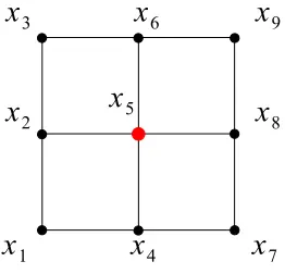
5.1 A 9-point local stencil. . . 71

5.2 CV formation in 2D. . . 72

5.3 Enumeration in a system of Nx ×Ny = 4×3 sub-domains of a

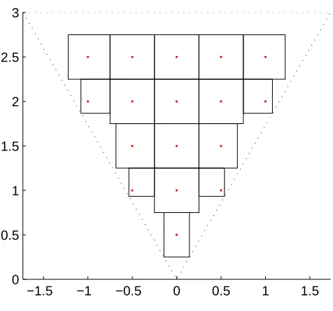
rectangular domain. . . 75 5.4 Enumeration in a system of 7 sub-domains of a triangular domain. 76 5.5 Algorithm of the parallel DD method using the local IRBF based

CV approach. . . 78

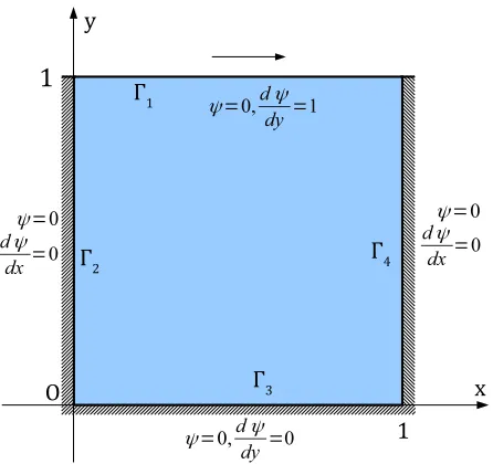
5.6 The square LDC fluid flow problem. Geometry and boundary con-ditions. No slip is assumed between the fluid and solid surfaces.

The top lid is moving from left to right with a speed of 1. . . 80

5.7 The square LDC ﬂuid ﬂow problem. Stream-function (ψ)

con-tours of the ﬂow for several Reynolds numbers Re = _{100, 400,

1000, 3200_} by the present parallel method using 4 sub-domains

for Re = 100,400,1000 and 2 sub-domains for Re = 3200 with

the speciﬁcations: grid 151_×151, ∆t = 10−3_, _ABCM

tol = 10−6,

CMtol = 10−6 and β = 2. . . 81

5.8 The square LDC ﬂuid ﬂow problem. Vorticity (ω) contours of the

ﬂow for several Reynolds numbers Re=_{100, 400, 1000, 3200_} by

the present parallel method using 4 sub-domains for Re = _{100,

400, 1000_}and 2 sub-domains for Re= 3200. The other

(16)

List of Figures xv

5.9 The square LDC fluid flow problem. Profiles of the u velocity

along the vertical centreline and thev velocity along the horizontal

centreline (solid lines) for several Reynolds numbers Re = _{100,

400, 1000, 3200_} by the present parallel method in comparison

with the corresponding Ghia’s results ( for u velocity and # for

v velocity). The parameters of the present method are given in

Fig. 5.7. . . 83

5.10 The square LDC fluid flow problem. Comparison between the parallel performance of the P-C and P-CV methods for several Reynolds numbers (Re= 100, 400, 1000 and 3200) with a grid of 151_×151: the efficiency, speed-up and simulation time of the two methods as a function of the number of CPUs. Other parameters are given in Tables 5.2 - 5.5. . . 89

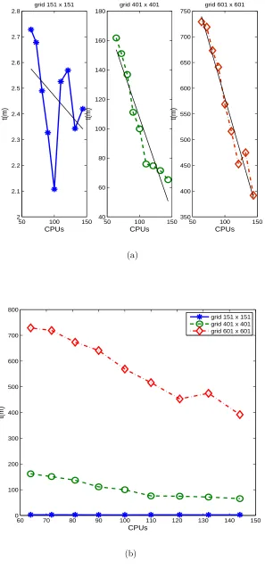
5.11 The square LDC fluid flow problem. Simulation time of the P-CV method withRe= 1000 using different grids: 151_×151, 401_×401 and 601_×601 as a function of the number of CPUs. . . 90

5.12 Triangular LDC ﬂow problem. Geometry and boundary condi-tions. P =√3, Q = 3. No slip is assumed between the ﬂuid and solid surfaces. The top lid is moving from left to right with a speed of 1. . . 91

5.13 CV formation in 2D. . . 92

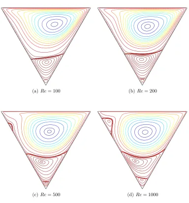
5.14 The triangular LDC fluid flow problem. Stream-function (ψ) con-tours of the flow for several Reynolds numbers by the present parallel method using 4 sub-domains with grid of 24697 points, ∆t = 5_×10−4_,_ABCM tol = 10−6, CMtol = 10−6 and β = 1. . . 93

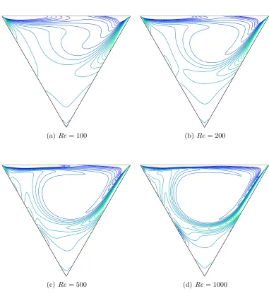
5.15 The triangular LDC fluid flow problem. Vorticity (ω) contours of the flow for several Reynolds numbers by the present parallel method. Other parameters are given in Fig. 5.14. . . 94

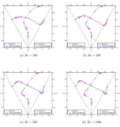
5.16 The triangular LDC fluid flow problem. Vorticity profiles along vertical line (x= 0) and horizontal line (y= 2) for several Reynolds numbers by the present parallel method in comparison with the corresponding Kohno and Bathe’s results ( for u velocity and # for v velocity). Other parameters of the present method are given in Fig. 5.14. . . 95

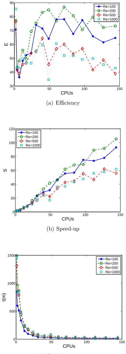
5.17 The triangular LDC fluid flow problem. Parallel performance of the P-CV methods for several Re using a grid of 24607 points: the efficiency, speed-up and simulation time as a function of the number of CPUs. Other parameters are given in Table 5.7. . . 98

6.1 2D 9-point stencil with x5 is the point under consideration. . . 103

6.2 Non-rectangular stencil . . . 107

6.3 Non-overlapping DD method in 2D . . . 108

6.4 Flowchart of parallel algorithm based on non-overlapping Dirichlet-Neumann DD method . . . 112

(17)

List of Figures xvi

6.6 The LDC ﬂuid ﬂow problem. Stream-function (ψ) contours of the

ﬂow for several Reynolds numbers (Re= 100, 400, 600 and 1000)

by the present parallel method using 16 CPUs with the speciﬁca-tions: grid 151_×151, ∆t= 10−3_,_CM[u]

tol = 10−6,ABCM [u]

tol = 10−6,

ABCM[

∂u ∂n]

tol = 10−6, θ = 0.45 andβ = 2. . . 114

6.7 The LDC fluid flow problem. Vorticity (ω) contours of the flow

for several Reynolds numbers (Re = 100, 400, 600 and 1000) by

the present parallel method using 16 CPUs. Other parameters are given in Fig. 6.6. . . 115

6.8 The LDC fluid flow problem. Profiles of the u velocity along

the vertical centreline (dashed lines) and the v velocity along the

horizontal centreline (solid lines) for several Reynolds numbers

(Re = 100, 400, 600 and 1000) by the present parallel method

in comparison with the corresponding Ghia’s results ( for u

ve-locity and # for v velocity). Parameters of the problem are given

in Fig. 6.6. . . 116 6.9 The LDC ﬂuid ﬂow problem. Performance of the present parallel

algorithm for several Reynolds numbers (100, 400, 600 and 1000)

with a grid of 151_×151: the eﬃciency, speed-up and simulation

time as a function of the number of CPUs. Other parameters are given in Tables 6.1, 6.2. . . 120 6.10 The LDC ﬂuid ﬂow problem. Comparison of execution times

be-tween the sequential computation and parallel computation using 25 CPUs . . . 121 6.11 The NC problem. Geometry and BCs. . . 122

6.12 The NC problem. A sample grid of 28_×28 points with 24

sub-domains. . . 123 6.13 The NC problem. Sub-domain formation and enumeration. . . 124 6.14 The NC problem. BCs on ABs of sub-domains. . . 124

6.15 The NC problem. Stream-function (ψ) contours (on the left) and

vorticity (ω) contours (on the right) of the ﬂow for several Rayleigh numbers using 24 sub-domains, grid 120_×120, ∆t= 10−4,CMtol[u]=

10−9_,_ABCM[u]

tol = 10−8, ABCM [∂u

∂n]

tol = 10−8,θ = 0.25 and β = 2. . 127

6.16 The NC problem. Temperature (T) contours (on the left) and

normal derivative of temperature ∂T

∂n along the inner circle (on

the right) of the ﬂow for several Rayleigh numbers, using 24 sub-domains, other parameters are given in Fig. 6.15. . . 128 6.17 The NC ﬂow problem. Performance of the present parallel

algo-rithm for several Rayleigh numbers: the eﬃciency, speed-up and simulation time with respect to the number of CPUs. Other pa-rameters are given in Table 6.5. . . 131 6.18 The NC ﬂow problem. Comparison of execution times between the

sequential computation and parallel computation using 24 CPUs . 132

(18)

List of Figures xvii

7.3 The 4:1 planar contraction flow problem. Sub-domains are over-lapping even though the overlapped zones are not shown. . . 141 7.4 The 4:1 contraction flow of Newtonian fluids. Stream-function

(ψ) contours of the ﬂow for several Reynolds numbers (Re =

{1,100,200_}) by the present parallel method using 20 sub-domains, grid 3, CMtol = 10−8, CMtolAB = 10−6, β = 2 and ∆t = 5×10−3

for Re=_{1,100_} and 10−3 _for _Re_{= 200. . . 143}

7.5 The 4:1 contraction ﬂow of Newtonian ﬂuids. Stream-function

(ψ) contours of the ﬂow for several Reynolds numbers (Re =

{300,400,500_}) by the present parallel method using 20 sub-domains, grid 3 with the speciﬁcationsCMtol = 10−8,CMtolAB = 10−6, β= 2

and ∆t = 10−3_{. . . 144}

7.6 The 4:1 contraction flow of Newtonian fluids. The efficiency (a), simulation time (b) and speed-up (c) of the present parallel method. Parameters are in given in Tables 7.2- 7.4 . . . 146

7.7 The 4:1 contraction ﬂow of Oldroyd-B ﬂuid. Stream-function (ψ)

contours of the ﬂow for W e = _{0.1, 0.2, 0.3_} by the present

par-allel method using 20 CPUs, grid 3, ∆t = 10−3_, _CM

tol = 10−8,

ABCMtol = 10−6 and β= 2. . . 148

contours of the ﬂow for W e = _{0.4,0.5_} by the present

paral-lel method using 10 CPUs, grid 2, ∆t = 10−3_, _CM

tol = 10−8,

ABCMtol = 10−6 and β= 2. . . 149

contours of the ﬂow for W e = _{0.8, 0.9, 1_} by the present

par-allel method using 1 CPU, grid 1, ∆t = 10−3_, _CM

tol = 10−8,

ABCMtol = 10−6 and β= 2. . . 150

7.10 The 4:1 contraction ﬂow of Oldroyd-B ﬂuid. τxx contours of the

ﬂow forW e=_{0.1, 0.2, 0.3_} with parameters given in Fig. 7.7. . 151

ﬂow forW e=_{0.4,0.5_} with parameters given in Fig. 7.8. . . 152

ﬂow forW e=_{0.8, 0.9, 1_} with parameters given in Fig. 7.9. . . 153

7.13 The 4:1 contraction ﬂow of Oldroyd-B ﬂuid. τxy contours of the

ﬂow forW e=_{0.4, 0.5_}with parameters given in Fig. 7.8. . . 155

ﬂow forW e=_{0.8, 0.9, 1_} with parameters given in Fig. 7.9. . . 156

7.16 The 4:1 contraction ﬂow of Oldroyd-B ﬂuid. τyy contours of the

ﬂow forW e=_{0.4,0.5_} with parameters given in Fig. 7.8. . . 158

flow forW e=_{0.8, 0.9, 1_} with parameters given in Fig. 7.9. . . 159 7.19 The 4:1 contraction flow of Oldroyd-B fluid. The efficiency (a),

(19)

List of Figures xviii

(20)

List of Tables

3.1 Comparison of various termination detection algorithms. M: the

number of basic messages, n: the number of processes, E: the

number of links, k: the number of failed processes. . . 37

4.1 2D problem with Dirichlet Boundary conditions. CPUs: number

of CPUs; ABCMtol: the tolerance of convergence measure on the

artiﬁcial interfaces; Ni: number of iterations; Nes: error norm

for the single domain CLIRBF method; Nep: error norm for the

parallel CLIRBF-DD method; Ts: sequential computation time

(second); Tp: parallel computation time (second). . . 53

4.2 2D problem with Neumann and Dirichlet Boundary conditions.

CPUs: number of CPUs; ABCMtol: the tolerance of convergence

measure on the artiﬁcial interfaces; Ni: number of iterations;Nes:

error norm for the single domain CLIRBF method;Nep: error norm

for the parallel CLIRBF-DD method; Ts: sequential computation

time (second); Tp: parallel computation time (second). . . 53

4.3 Parallel computation of the LDC ﬂuid ﬂow problem with Re =

100; CPUs: number of CPUs; ∆t: time step; CMtol: tolerance of

convergence measure at interfaces; Ni: number of iterations; Tp:

parallel computation time (minutes); CM: average convergence

measure of the whole analysis domain. . . 63

4.4 Parallel computation of the LDC ﬂuid ﬂow problem with Re =

400; CPUs: number of CPUs; ∆t: time step; CMtol: tolerance of

convergence measure at interfaces; Ni: number of iterations; Tp:

parallel computation time (minutes); CM: average convergence

measure of the whole analysis domain. . . 64

4.5 Parallel computation of the LDC problem withRe= 1000; CPUs:

number of CPUs; ∆t: time step; CMtol: tolerance of convergence

measure at interfaces; Ni: number of iterations; Tp: parallel

com-putation time (minutes);CM: average convergence measure of the

whole analysis domain. . . 65

4.6 Parallel computation using the present method for the LDC

prob-lem with Re = 100, grid 101_×101 and ∆t = 1.E₋5. nx×ny:

grid points; CP Us: number of CPUs; CN: condition number

of the system matrix; CMp: average convergence measure of the

whole analysis domain; Ni: number of iterations on the whole

do-main; Tcmp: computational time for one iteration in sub-domain

(seconds); Tcmm: total communication time (minutes); Tp: total

parallel computation time (minutes). . . 66

(21)

List of Tables xx

5.2 The square LDC ﬂuid ﬂow problem. Comparison between parallel

CV (P-CV) and parallel collocation (P-C) methods withRe= 100,

grid 151_× 151, dt = 10−3_, _ABCM

tol = 10−6, CMtol = 10−6,

β = 2. CPUs: number of CPUs; Ni: number of iterations; Tp:

parallel computation time (minutes); S: speed-up; E: eﬃciency.

The observed super-linear speed up can be explained in terms of

reduced matrix condition numbers (see main text). . . 84

5.3 The square LDC ﬂuid ﬂow problem. Comparison between P-CV

and P-C methods with Re= 400, grid 151×151. CPUs: number

of CPUs; Ni: number of iterations; Tp: parallel computation time

(minutes); S: speed-up; E: eﬃciency. Other parameters are given

in Table 5.2. . . 85

and P-C methods withRe= 1000, grid 151_×151. CPUs: number

in Table 5.2. . . 86

and P-C methods withRe= 3200, grid 151_×151. CPUs: number

in Table 5.2. . . 87

5.6 The square LDC ﬂuid ﬂow problem. Condition numbersCNω and

CNψ in single and parallel solutions with Re = 100 and grid =

151_×151. CPUs: number of CPUs (sub-domains). . . 88

5.7 The triangular LDC ﬂuid ﬂow problem. Results by the present

P-CV method with grid of 24697 points, ∆t = 5.E₋04,ABCMtol =

10−6_,_CM

tol = 10−6, β = 1. CPUs: number of CPUs; Ni: number

of iterations; Tp: parallel computation time (minutes); S:

speed-up; E: eﬃciency. . . 96

6.1 The LDC ﬂuid ﬂow problem. Parallel performance with grid 151_×

151, ∆t = 10−3_, _CM[u]

tol = 10−6, ABCM [u]

tol = 10−6, ABCM [∂u

∂n]

tol =

10−6_,_θ_{= 0}_._{45 and}_β _{= 2. CPUs: number of CPUs (sub-domains);}

Ni: number of iterations; Tp - parallel computation time (minutes)

on parallel CPUs, i= 1 for single CPU; S - speed-up; E - eﬃciency.117

6.2 The LDC ﬂuid ﬂow problem. Parallel performance with grid 151_×

151, ∆t = 10−3_, _CM[u]

tol = 10−6, ABCM [u]

tol = 10−6, ABCM [∂u

∂n]

tol =

10−6_,_θ _{= 0}_._{45 and}_β _{= 2. CPUs - number of CPUs (sub-domains);}

Ni - number of iterations;Tp - parallel computation time (minutes)

on parallel CPUs except for the case with 1 CPU which is

(22)

List of Tables xxi

6.3 The LDC ﬂuid ﬂow problem. Comparison between computation time and communication time in parallel program and total time between parallel program and sequential program. Parallel

pro-gram runs on 25 CPUs. Re is Reynolds number, Tcmm:

com-munication time (minute), Tcmp: computation time (minute), Tp:

parallel computation time (minutes), % Tcmm: percentage of

com-munication time in total time, Ts: sequential computation time

(minutes), Tn: normalised time, E: eﬃciency . . . 119

6.4 The NC problem. Comparison of average Nusselt numbers. Present results are obtained by a parallel algorithm with 24 CPUs . . . . 126

6.5 The NC problem. Parallel performance with Ra= 104_{, grid 120}_×

120, ∆t = 10−4_, _CM[u]

tol = 10−9, ABCM [u]

tol = 10−8, ABCM [∂u

∂n]

tol =

10−8_,_θ _{= 0}_._{25 and}_β _{= 2. CPUs: number of CPUs (sub-domains);}

Ni: number of iterations;Nuoaverage Nusselt number on the outer

square (cold wall);Nui average Nusselt number on the inner circle

(hot wall); t(m): elapsed time (minutes); S: speed-up; E: eﬃciency.129

120, other parameter can be seen in Table 6.5. . . 129

120, other parameter can be seen in Table 6.5. . . 130 6.8 Condition number of system matrix in LDC and NC problems with

respect to number of CPUs (sub-domains) . . . 130 6.9 The NC ﬂow problem. Comparison between the computation time

and communication time in parallel program, and the total time between parallel computation and sequential computation.

Paral-lel program using 24 CPUs. Ra: Rayleigh number,Tcmm:

commu-nication time in minutes, Tcmp: computation time in minutes, Tp:

computation time (minutes) on parallel CPUs, %Tcmm: percentage

of communication time in total time, Ts: computation time

(min-utes) on single CPU, Tn: normalised time (minutes), E: eﬃciency 130

7.1 Grid characteristics . . . 142 7.2 The 4:1 contraction ﬂow of Newtonian ﬂuids. Parallel performance

for Re = _{1,100_} with grid 3, ∆t = 5_× 10−3_, _CM

tol = 10−8,

ABCMtol = 10−6, and β = 2. p: number of CPUs; Ni: number of

iterations; Tp: parallel computation time (minutes); S: speed-up;

E: eﬃciency. Tp with 20 CPUs is used for reference. . . 145

7.3 The 4:1 contraction ﬂow of Newtonian ﬂuids. Parallel performance for Re=_{200,300_}with grid 3, ∆t = 10−3_{, other parameters are}

given in Table 7.2. Tp with 20 CPUs is used for reference. . . 145

7.4 The 4:1 contraction ﬂow of Newtonian ﬂuids. Parallel performance for Re=_{400,500_}with grid 3, ∆t = 10−3_{, other parameters are}

given in Table 7.2. Tp with 20 CPUs is used for reference. . . 147

7.5 The 4:1 contraction ﬂow of Oldroyd-B ﬂuid. Parallel performance

with grid 3, ∆t = 10−4_, _CM

tol = 10−8, ABCMtol = 10−6, and

β = 2. Ni - number of iterations; Tp - parallel computation time

(minutes); S - speed-up; E - eﬃciency. Tp with 20 CPUs is used

(23)

List of Tables xxii

7.6 The 4:1 contraction ﬂow of Oldroyd-B ﬂuid. Parallel performance

with grid 3, ∆t = 10−4_, _CM

tol = 10−8, ABCMtol = 10−6, and

β = 2. Ni - number of iterations; Tp - parallel computation time

(minutes); S - speed-up; E - eﬃciency. Tp with 20 CPUs is used

as reference. . . 148 7.7 The 4:1 contraction ﬂow of Oldroyd-B ﬂuid. Parallel performance

with grid 2, ∆t = 10−3_, _CM

tol = 10−8, CMtol = 10−6, and β = 2.

Ni - number of iterations;Tp - parallel computation time (minutes)

except for the case with 1 CPU which is non-parallel andTp ≡Ts;

(24)

Chapter 1

Introduction

In this chapter, an introduction to the thesis is presented. Firstly, the motivation, significance and objectives of the thesis are discussed. Secondly, the fundamental equations that govern the motion of Newtonian and non-Newtonian fluids, are presented, followed by a review of numerical methods for fluid flow analysis. Lastly, an outline of the thesis is given at the end of this chapter.

1.1

Motivation, significance and objectives

(25)

1.2. Fluid dynamics 2

this thesis are based on Domain Decomposition methods (DDM) and Integrated Radial Basis Function (IRBF) method, achieving the following advantages: (i) ease of load balancing among CPUs; (ii) low message complexity thanks to the fact that each CPU communicates with only four neighbouring CPUs; and (iii) high scalability associated with a distributed memory parallel computing model.

In a distributed system, if a process terminates arbitrarily, other processes will not be able to exchange data with it and the whole system might hang up for-ever. Hence, every process has to be aware of the status of all other processes so that it can terminate properly. This is actually an important research topic in distributed computing called Distributed Termination Detection (DTD) (Di-jkstra and Scholten, 1980). Although there is a number of DTD algorithms available in the literature, it is necessary to develop a new DTD algorithm that can be incorporated eﬃciently into parallel methods based on DD and IRBF. The presently proposed DTD algorithm has four main advantages including sym-metric detection mechanism, decentralised control, low message complexity and optimal termination detection delay.

The developed parallel methods and DTD algorithm can be applied to solve various CFD problems. This will give researchers a powerful and ﬂexible tool to deal with problems that are currently diﬃcult to investigate because of the limitation of computing resource. Furthermore, the DTD algorithm has a broader range of applications as it can be used in many distributed systems other than CFD without any major alteration.

In summary, main objectives of the thesis includes

1. Develop a DTD algorithm for an eﬃcient and proper termination of parallel methods;

2. Develop parallel methods based on DD method and IRBF method to solve CFD problems;

3. Apply the developed methods to solve various CFD problems, including ﬂows of Newtonian and Newtonian ﬂuids in both rectangular and non-rectangular domains.

1.2

Fluid dynamics

(26)

1.2. Fluid dynamics 3

mass, the conservation of momentum and the conservation of energy. For an incompressible ﬂuid, the conservation of mass is expressed by

∇ ·v= 0, x_∈Ω, (1.1)

wherevis the velocity vector,xthe position vector, and Ω the domain of interest.

The conservation of momentum is described as

ρ ∂v

∂t +v· ∇v

!

=_{∇ ·}σ+ρg, x∈Ω, (1.2)

where t is the time, ρ the density, σ the total stress tensor and g the force per

unit mass due to gravity (Tanner, 2000; Reddy and Gartling, 1994).

The total stress tensor is given by σ = −pI +τ, where p is the hydrostatic

pressure, I the identity tensor and τ the extra stress tensor. Eq. (1.2) can now

be rewritten as

ρ ∂v

∂t +v· ∇v

!

=_−∇p+_{∇ ·}τ +ρg, x∈Ω. (1.3)

The pressure term and gravity term can be combined into one term called

modi-ﬁed pressure, _∇P =_∇p₋ρg, and Eq. (1.3) becomes

ρ ∂v

∂t +v· ∇v

!

=_−∇P +_{∇ ·}τ, x∈Ω. (1.4)

The mechanical behaviour of a ﬂuid can be described by a constitutive equation. For Newtonian ﬂuids, the constitutive equation has the form of

τ = 2η0D, (1.5)

where η0 is the constant viscosity, and D the rate of deformation tensor, deﬁned

as D= 1

2

∇vT +_∇v.

For non-Newtonian ﬂuids, many diﬀerent constitutive models have been devel-oped. Some of them are given as follows.

Upper-Convected Maxwell (UCM) model

τ +λ₁τ∇= 2η0D, (1.6)

whereλ1 is the characteristic relaxation time of the ﬂuid and the upper-convected

derivative ∇[] is deﬁned as

∇ [] = ∂[]

∂t +v· ∇[]−(∇v)

T

·[]−[]· ∇v. (1.7)

Oldroyd-B model

τ +λ₁τ∇= 2η₀

D+λ2

∇

D

(27)

1.3. Numerical methods 4

where λ2 is the characteristic retardation time of the ﬂuid. Let α be the ratio

of the retardation time to the relaxation time (α = λ2/λ1). When α = 0 the

Oldroyd-B model yields the UCM one.

The extra stress tensor τ consists of two components, the solvent and polymeric

contributions.

τ = 2η_sD+τ_v, (1.9)

where ηs is the solvent viscosity and τ_v the elastic stress, which is given by

τ_v+λ₁τ∇_v = 2η_pD, (1.10)

where ηp is the polymeric viscosity, η0 =ηs+ηp, ηs =αη0, and ηp = (1−α)η0.

As found in Eq. (1.9) if the value ofηsis equal to zero, thenτ =τ_v, the

Oldroyd-B model becomes UCM one (Covas et al., 1995; Phan-Thien and Tanner, 1977).

Giesekus-Leonov model

τ_v+λ₁τ∇_v−λ1

2ηp

τ_vτ_v = 2η_pD. (1.11)

Phan-Thien Tanner (PTT) model 1

exp λ1ε

ηp

tr(τ_v)

!

τ_v+λ₁τ∇_v+ξλ₁(Dτ_v +τ_vD) = 2η_pD, (1.12)

where ε and ξ are the material parameters, and ‘tr’ denotes the trace operation.

Phan-Thien Tanner (PTT) model 2

1 + λ1ε

ηp

tr(τ_v)

!

τ_v+λ₁τ∇_v+ξλ₁(Dτ_v+τ_vD) = 2η_pD, (1.13)

where the coeﬃcients are deﬁned as before. For more details about PTT models, please refer to (Phan-Thien, 1978, 1984; Tanner, 2000).

1.3

Numerical methods

In practical problems, the above governing equations can rarely be solved ana-lytically. Instead, their solution is normally sought in the form of approximation given by numerical methods. Common numerical methods are presented brieﬂy below.

1.3.1 Finite Difference method (FDM)

(28)

1.3. Numerical methods 5

points (Smith, 1978). The derivatives of the function are approximated using the nodal values of the function. The diﬀerential equation is discretised into a system of algebraic equations whose unknowns are the nodal function values. The method is well-known for its speed thanks to the tri-diagonal form of the system matrix (Conte and Dames, 1958; Gupta and Manohar, 1979; Bjorstad, 1983). However, the method has low accuracy due to the fact that the conservation is not enforced inherently. High-order schemes have been successfully introduced to increase the accuracy of the method, such as compact FD scheme (Lele, 1992; Li et al., 1995), high-order FD upwind scheme (Ferreira et al., 2009), pseudo-spectral FDM (Pilitsis and Beris, 1989). More details can be found in Mitchell and Griﬃths (1980) and Crochet et al. (1984), for example.

1.3.2 Finite Volume method (FVM)

In finite volume method, the computation domain is divided into contiguous con-trol volumes (CV). The governing equation is integrated over the whole CV. By applying Green formulae, the surface integration is transformed to line integra-tion. With appropriate quadrature rule, the line integration is approximated in terms of nodal values, i.e., a linear equation is achieved (Patankar, 1980; Huilgol and Phan-Thien, 1997). FVM is conservative by construction (Eymard et al., 2000). In addition, the method is suitable for many types of grid. However, FVMs of order higher than second are more difficult to develop because FVM requires three levels of approximation, namely interpolation, differentiation and integration.

1.3.3 Finite Element method (FEM)

Finite element method is the favoured discretisation method in structural me-chanics (Hughes, 1987b; Rannacher, 1999; Reddy, 2005). Thanks to the ability to model singularities through mesh refinement, FEMs have been used in many non-Newtonian fluid flow simulations (Yurun and Crochet, 1995; Fan et al., 1999; Sun et al., 1999). However, the matrices of the linearised equations are not well structured so FEM normally requires highly efficient solution methods (Pastor et al., 1991). In addition, generating a FE mesh is a costly process and the solu-tion has a slow convergence in high gradient regions (Pastor et al., 1991; Emdadi et al., 2008). Galerkin FEM and mixed FEM (Baaijens, 1998) and the streamline upwind Petrov-Galerkin (SUPG) (Brooks and Hughes, 1982; Hughes, 1987a) are among the most popular schemes.

1.3.4 Boundary Element method (BEM)

(29)

1.4. Outline of the Thesis 6

Hence, BEM can be more eﬃcient than other methods in terms of computational resources for problems where the surface-to-volume ratio is small. BEM is very useful for problems where the physically relevant data are given not by the so-lution in the interior of the domain but rather on the boundary (Brebbia et al., 1984). The accuracy of the solution by BEM on the boundary is superior to those by FEM. However, BEM is only applicable to problems, for which a Green’s func-tion is available. Thus, problems with inhomogeneities or governed by non-linear diﬀerential equations normally are not solved straightforwardly by BEM itself but rather in combination with other methods. BEM normally produces fully pop-ulated matrices. As a result, memory and computation time required by BEM will grow as the square of the problem size (Tanner and Xue, 2002).

1.3.5 Radial Basis Function (RBF) method

Radial Basis Functions have traditionally been used to provide a continuous in-terpolation of scattered data sets (Franke, 1982; Haykin, 1999). Details on several well-known radial basis functions are given in Appendix A. For differential RBF (DRBF) method, the function values are first approximated by weighted RBFs. Such closed form can then be differentiated analytically to obtain derivatives of the function. On the other hand, in integrated RBF (IRBF) method the highest-order derivatives of the ODE/PDE is approximated by weighted RBFs first. Subsequently, its lower-order derivatives and function values are obtained through integration (Mai-Duy and Tran-Cong, 2001). RBF method is considered as a high order method (Kansa, 1990a). Furthermore, RBF method is able to solve problems with complex boundary. The main drawback of RBF methods is the fact that coefficient matrices are fully populated and may be ill-conditioned. To overcome these problems, local and compact schemes have been proposed (Shu et al., 2003; Lee et al., 2003; Kosec and Sarler, 2008; Bourantas et al., 2010; Mai-Duy et al., 2011). Details on RBF methods will be presented in the Chapter 2.

1.4

Outline of the Thesis

The remaining of the thesis is organised as follows.

• Chapter 2 consists of four parts describing the basic tools used in the present research project. The ﬁrst part is to present the IRBF methods including compact local IRBF schemes. The second part is to review the DD method. The third part is to present the parallel computation together with the challenges to parallel performance. Finally, in the last part, the termination detection in parallel algorithm is discussed.

(30)

1.4. Outline of the Thesis 7

• Chapter 4 reports a parallel method achieved by combining the overlapping DD method and the CLIRBF approach. The method is veriﬁed by problems with available analytic solution and the benchmark problem of lid-driven cavity ﬂow (Pham-Sy et al., 2013).

• Chapter 5 is to develop parallel method based on local IRBF Control Vol-ume method and overlapping DD method. The method is veriﬁed through the simulation of the lid-driven ﬂows in both rectangular and triangular cavities (Pham-Sy et al., 2014).

• Chapter 6 reports a parallel method based on non-overlapping DD method and compact local IRBF approach. The method is veriﬁed by solving two benchmark problems, which are the lid-driven cavity ﬂow and the natural convection in concentric annuli (Pham-Sy et al., 2015b).

• Chapter 7 is to demonstrate the efficiency of the present parallel methods by simulating the benchmark 4:1 planar contraction flow of Newtonian and Oldroyd-B fluids.

(31)

Chapter 2

Fundamental background

This chapter describes several basic tools, which are the background for the nu-merical methods and their parallelisation developed in the present work. These tools are the Radial Basis Function (RBF) based approximation methods, the Do-main Decomposition (DD) methods together with parallel programming and the Distributed Termination Detection (DTD) algorithms. In this dissertation, the integrated RBF approaches (IRBF), which are considered as numerical methods for function approximation and numerical solution of partial differential equa-tions (PDEs), will be coupled with the DD technique in both collocation and control volume (CV) approaches. The DD techniques help methods take advan-tage of high performance computing (HPC) capability for the simulation of the fluid flows problems.

2.1

Radial Basis Function method

(32)

2.1. Radial Basis Function method 9

u(x) = n

X

i=1

wigi(x), (2.1)

∂k_u₍_x₎

∂xk j

=Xn

i=1

w[xj]

i h [k]

[xj]i(x), (2.2)

where xj is the j-component of x (j = 1,2); superscript [k] denotes the order of

the derivatives of u (k = 1,2), andh[_[_xk]_j_]_i(x) = ∂ k_g

i(x)

∂xk j

.

More recently, Mai-Duy and Tran-Cong (2001) proposed the idea of the inte-grated RBF method. Within the IRBF based methods, the highest order of the derivatives in an ODE/PDE is approximated ﬁrst and, subsequently, its lower-order derivatives and the function itself are obtained through integration. This method can yield very accurate solutions using a relatively small number of grid nodes (Mai-Duy and Tran-Cong, 2003). IRBF methods can be global, local or compact local.

Consider the Poisson’s equation in 2D.

∇2u(x) =f(x), x_∈Ω, (2.3)

where uis the ﬁeld variable; xthe position vector; Ω the considered domain and

f a known function of x.

The domain of interest is discretised using a Cartesian grid. Let nx and ny be

the numbers of grid lines in the x- and y-directions, respectively. Suppose the

domain is rectangular, the total number of grid nodes will be n =nx×ny.

2.1.1 Global IRBF

Two dimensional IRBF method (2D-IRBF)

In the global 2D-IRBF method, the dependent variable u and its derivatives are

approximated using all grid nodes.

For the Poisson’s equation (2.3), the highest order derivatives of the PDE, i.e. second order, are approximated by a weighted set of RBFs as

∂2u(x)

∂x2 j = n X i=1

w[xj]

i g [xj]

i = n

X

i=1

w[xj]

i G [2]

[xj]i(x), (2.4)

where xj is the j-component of x (j = 1,2); {wi}ni=1 the set of weights and

{gi(x)}ni=1 the set of RBFs. The superscript [.] is used to indicate the associated

derivative order. The MQ-RBF is used in this work and given by

Gi(x) =

q

(33)

where _{ci}ni=1 is a set of centres and {ai}ni=1 a set of MQ-RBF widths.

To obtain ﬁrst-order derivatives and ﬁeld variable, Eq. (2.4) is integrated succes-sively with respect to xj as follows.

∂u(x)

∂xj

=Xn

i=1

w[xj]

i G [1]

[xj]i(x) +C

[xj]

1 (xk), k 6=j, (2.5)

u[xj](_x) =

n

X

i=1

w[xj]

i G [0]

[xj]i(x) +xjC

[xj]

1 (xk) +C [xj]

2 (xk), k 6=j, (2.6)

where G[1]_[_x_j_]_i(x) =

Z

G[2]_[_x_j_]_i(x)dxj, G[0]_[xj]i(x) =

Z

G[1]_[_x_j_]_i(x)dxj, and C [xj]

1 (xk) and

C[xj]

2 (xk) are constants of integration which are functions of the variablexk,k6=i.

Collocating equations (2.4) - (2.6) at grid points _{xi}ni=1 yields

∂2_u_e

∂xj

=_G[2]

xjwexj, (2.7)

∂ue

∂xj

=_G[1]

xjwexj, (2.8)

e

uxj =G

[0]

xjwexj, (2.9)

with

e

wxj =

w[xj]

1 , w [xj]

2 ,· · · , w[nxj], C [xj]

1 , C [xj]

2

T

,

e

uxj =

u[xj]

1 , u [xj]

2 ,· · · , u[nxj]

T

,

∂k_u_e

∂xk j

= ∂ku1

∂xk j ,∂ k_u 2 ∂xk j ,_{· · ·},∂ k_u n ∂xk j !T ,

where u[xj]

i =u[xj](xi) (i= 1,2,· · · , N); G[2],Gx[1]j and G

[0]

xj are known matrices.

One dimensional IRBF method (1D-IRBF)

One dimensional IRBF method shares the same principle as 2D-IRBF. The only

diﬀerence is that, in 1D-IRBF the dependent variable u and its derivatives are

approximated using nodes on a single line along the directions. 1D-IRBF method

uses only nx or ny nodes, compare to n nodes of 2D-IRBF, to construct the

ap-proximation of a value at a given point. As a result, a much sparser approxima-tion matrix is obtained. Sparse matrices generally have better condiapproxima-tion number. They are also less expensive to compute than dense matrices. The

approxima-tion of a PDE now consists of (i) using IRBFs to approximate the variable u and

its derivatives along a grid-line, and (ii) applying Kronecker tensor product to construct the approximation matrix for derivatives over a 2D domain.

For example, consider an xj-gridline, which runs parallel to the xj-axis. For

simplicity, the grid nodes are numbered from left to right, started with x1 and

(34)

The second order derivative of the PDE at an arbitrary point in the considered line is approximated as follows.

∂2_u₍_x₎

∂x2 j = nj X i=1

wigi = nj

X

i=1

wiGi(x). (2.10)

The ﬁrst-order derivatives and ﬁeld variable are then obtained as follows. ∂u ∂xj = nj X i=1

wiG [1]

i (x) +C1, (2.11)

u=

nj

X

i=1

wiG[0]i (x) +C1xj+C2. (2.12)

Collocating equations (2.10) - (2.12) at grid points_{xi} nj

i=1 yields

∂2_u_e

∂xj

=_G[2]_w_e_, _(2.13)

∂ue

∂xj

=_G[1]_w_e_, _(2.14)

e

u=_G[0]we, (2.15)

with

e

w = w1, w2,· · · , wnj, C1, C2

T

,

e

u = u1, u2,· · · , unj

T

,

∂k_u_e

∂xk j

= ∂ku1

∂xk j ,∂ k_u 2 ∂xk j ,_{· · ·} ,∂ k_u nj ∂xk j !T ,

where ui = u(xi) (i = 1,2,· · · , nj); G[2],G[1] and G[0] are known matrices of size

nj×(nj + 2) as presented below.

G[k](k = 1,2,3) =

       

G[1k](x1) G [k]

2 (x1) · · · G[nkj](x1) a

[k] 1 b

[k] 1

G[1k](x2) G [k]

2 (x2) · · · G[2]nj(x2) a

[k] 2 b

[k] 2

... ... . .. ... ... ...

G[₁k](xnj) G

[k]

2 (xnj) · · · G

[k]

nj(xnj) a

[k] nj b

[k] nj         , where

a[1k], a [k]

2 , · · · , a[nkj]

T =           

0, 0, _{· · ·} , 0 T, k= 2

1, 1, _{· · ·} , 1 T, k= 1

xj1, xj2, · · · , xjnj

T

, k = 0

and

b[1k], b [k]

2 , · · · , b[nkj]

T =     

0, 0, _{· · ·} , 0 T , k = 1,2

(35)

2.1.2 Local and compact local IRBF

As stated in Kansa (1990a), although the global RBF methods are proved to have better accuracy in approximating a function, they are time-consuming and require large storage. More importantly, when the number of collocation points increases, the system matrix becomes ill-conditioned. To overcome these drawbacks, several solutions have been suggested including local RBF based methods (Mai-Duy and Tanner, 2007; Mai-Duy et al., 2011) and domain decomposition (DD) methods (Beatson et al., 2001; Tran et al., 2009). The diﬀerence between local and global IRBF methods is that in local methods, the approximation of a function at a grid node involves a small number of surrounding nodes only.

However, local IRBF methods are less accurate as the approximation is based on a set of local points rather than the whole grid. To recover the loss of accuracy, compact schemes have been introduced (Mai-Duy et al., 2011; Hoang-Trieu et al., 2012; Thai-Quang et al., 2012). In this work, the 2D-IRBF compact scheme proposed in Mai-Duy et al. (2011) is employed and presented in details.

For 2D problems, a 9-point stencil scheme is applied to overcome the problem of ill-conditioned system matrix, which is an inherent issue in the global approach. According to this scheme, a local 9-point stencil for an arbitrary grid-point xi,j

(2_≤i_≤nx−1; 2≤j ≤ny −1) is described as follows.

  

xi−1,j+1 xi,j+1 xi+1,j+1 xi₋1,j xi,j xi+1,j xi₋1,j₋1 xi,j₋1 xi+1,j+1

  .

For simplicity, a speciﬁc local stencil is used here as

  

x3 x6 x9 x2 x5 x8 x1 x4 x7

  ,

Applying the 2D-IRBF procedure to this stencil leads to a system of algebraic equations for unknown nodal values of the ﬁeld variable as follows.

e u e 0 ! = " G[0] x , O

G[0]

x , −Gy[0]

#

| {z }

C e wx e wy !

=_C wex

e

wy

!

, (2.16)

where _C is the conversion matrix, wex and wey the RBF weight vectors of length

15;ue the vector of length 9, and₀e_{the zeros vector of length 9;} _O_{the zeros matrix}

of dimension 9_×15, and _G[0]

x and Gy[0] the known matrices of dimensions 9×15.

Furthermore, ue, wex and wey are given by

e

u= (u1, . . . , u9)T, (2.17)

e

wx = (wx1, . . . , wx9, C x

1(y1), C1x(y2), C1x(y3), C2x(y1), C2x(y2), C2x(y3))T, (2.18)

e

wy = (wy1, . . . , wy9, C y

(36)

2.1. Radial Basis Function method 13 G[0] x =                        

G[0]_[_x_]1(x1) _{· · ·} G[0]_[_x_]9(x1) x1 0 0 1 0 0

G[0]_[_x_]1(x2) · · · G[0][x]9(x2) 0 x2 0 0 1 0

... . .. ... 0 0 x3 0 0 1

... . .. ... x4 0 0 1 0 0

... . .. ... 0 x5 0 0 1 0

... . .. ... 0 0 x6 0 0 1

... . .. ... x7 0 0 1 0 0

... . .. ... 0 x8 0 0 1 0

G[0]_[_x_]1(x9) _{· · ·} G[0]_[_x_]9(x9) 0 0 x9 0 0 1

                        , (2.20) G[0] y =                        

G[0]_[_y_]1(x1) _{· · ·} G[0]_[_y_]9(x1) y1 0 0 1 0 0

G[0]_[_y_]1(x2) _{· · ·} G[0]_[_y_]9(x2) y2 0 0 1 0 0

... ... ... y3 0 0 1 0 0

... ... ... 0 y4 0 0 1 0

... ... ... 0 y5 0 0 1 0

... ... ... 0 y6 0 0 1 0

... ... ... 0 0 y7 0 0 1

... ... ... 0 0 y8 0 0 1

G[0]_[_y_]1(x9) _{· · ·} G[0]_[_y_]9(x9) 0 0 y9 0 0 1

                        , (2.21)

where G[0]_[_x_]_i and G[0]_[_y_]_i (i = 1..9) were deﬁned in Section 2.1.1 in the x and y -directions and xi, yi are the two components of xi. It is noted that in Eq. (2.16)

e

u= [_G[0] x ,O]

e

wx

e

wy

!

is obtained by collocating the ﬁeld variable over a local stencil, and

e

0= [_G[0]

x ,−Gy[0]]

e

wx

e

wy

!

is derived from the consistency conditio