Abstract—In this work a boundary element formulation for the analysis of plate-beam interaction is used in the analysis of practical building slabs and waffle slab. This formulation uses a boundary element with three degrees of freedom per node and the beam element is replaced by their actions on the plate, that is, a distributed load and end of element forces. From the solution of the differential equation of a beam with linearly distributed load the plate-beam interaction tractions can be written as a function of the nodal values of the beam. With this transformation a final system of equation in the nodal values of displacements of plate boundary and beam nodes is obtained and from it, all unknowns of the plate-beam system are obtained. The results show an excellent agreement with those from the a finite element analysis.
Index Terms—Boundary element method, plates in bending, beams, stiffners
I. INTRODUCTION
HE boundary element method was first applied to the analysis of buildings slabs by BÉZINE [1]) that analyzed the problem of plates with internal support that could be used to simulate a plate supported on rigid columns. Since then, several authors have developed formulations for the analysis of buildings slabs via the Boundary Element Method, BEM, [2,3,4,5,6,7]. In the usual formulation of the boundary element method for plates in bending the nodal parameters of the boundary elements are the displacements w and its derivative w
n
. As each beam’s
node has three nodal parameters the compatibility of displacements and rotations of nodes belonging to the beam and the boundary of the plate are hard to manage, requiring a re-organization of the final matrix of the system of equations generating special lines at the end of this system for the nodal parameters that do not coincide with those of the contour of the plate.
Manuscript received January 20th, 2015 revised March 2nd, 2015. This work was supported by the research council CNPq .
C. J. Oliveira is with Positivo University, Curitiba, PR,81280-330, Brazil, e-mail: [email protected]
J. B. Paiva is with the School of Engineering of São Carlos- University of São Paulo, São Carlos, SP, 13566-590, Brazil, e-mail:[email protected]
A. V. Mandonça is with Federal University of Paraiba, Civil
To solve this problem a BEM formulation with three nodal parameters was proposed,[8,9] but keeping Kirchhoff’s thin plates hypothesis [10]. With this formulation coupling the plate with beams and columns is much simpler. However in this case the connection of the plate with the beam is made exclusively by means of vertical forces at the nodes of the finite elements. Due to this punctual forces the bending moments at internal connecting plate-beam nodes are infinite, represented the solution of the differential equation of plates.
In this work, a new boundary element formulation for the analysis of the plate-beam interaction is presented, in which the plate is modeled by the formulation referred to above and the beam is replaced by its actions on the plate, a distributed load and forces at its ends [11,12].
In this formulation each beam element has three nodes, each with two nodal values, w and ∂w/∂sb, and the
transverse displacement of the beam is approximated by a fifth degree polynomial that represents the analytical differential equation solution for a beam under transverse loading with linear variation. As the interaction forces between the beam and the plate can be written as a function of transverse displacement and as it is written as a function of the nodal parameters, integral equations for the plate-beam coupling can be written in terms of the nodal displacements of the plate and the beam. By imposing the boundary conditions and solving the system of equations, the displacements and tractions on the beams and plate can readily be calculated.
This formulation was then used in the analysis of basic plates stiffened with beams and the results were excellent. However the formulation needed to be tested for more complex problems, such as plates with beams not parallel to its sides and also in usual building structures, such as waffle slabs.
This work presents the integral equations for the plate and the solution of the beam and its coupling and then show results obtained in the analysis of plates with non-parallel beams and also for a typical building floor designed as waffle slab. The results are compared with those obtained by the finite element method demonstrating excellent agreement and confirmed that this tool can be effectively used in the analysis of building floors slabs.
II. INTEGRAL EQUATIONS
For a plate in bending with concentric beams, Figure 1, the following boundary integral equations can be written, employing the alternative formulation of Boundary Element Method (BEM) with three nodal displacement parameters [8,9] in which the beam is replaced by the plate-beam interaction tractions(Fig. 1 (II)):
Boundary Element Analysis of Building Slabs
Charles Jaster de Oliveira, João Batista de Paiva, Ângelo Vieira Mendonça
Fig. 1. Plate and beam: coordinate systems and interface tractions 1 3 * ( ) ( ) ( , ) ( ) ( , ) ( ) ( , ) ( ) ( ) ( ) ( , ) ( ) ( , ) ( ) ( ) ( , ) ( ) ( , ) ( ) ( ) ( , ) ( ) ( , ) ( , ) c g n n
n s n
N
n c i c i
i
g b
b i i i i
b
w
K S w S q S Q w Q m S Q Q
n w
m S Q Q d Q V Q w S Q
s
w
m Q S Q d Q R Q w S Q
n
g q w S q d q P q w S q d S q
w
V w S q M S q
s
* * ( , ) ( , ) k k k k bV w S q
w
M S q
s
…(1) where w, mn and Vn are, respectively, the transverse
displacement, the bending moment and the equivalent shear force along the boundary; g(q) and Ωg are the transverse
load and the surface where it is applied; p3(q), Vi, Vk, Mi and
Mk are tractions at the plate-beam interface and Sb is the
coordinate along each beam element axis. The symbol * is used here to indicate fundamental solution.
From equation (1) the integral representation of the derivative of the displacement with respect to a directionms,
of a system of coordinates (ms,us), can be derived as
follows: 1 ( , ) ( ) ( , ) ( ) ( , ) ( ) ( , ) ( , ) ( ) ( ) c n
1 2 s
S S n ns S S * * n n S S N ci ci s s i q
S Q w Q
w w
(S) (S)+ (S) (S)+ m
K K
m u
m w m w
S Q Q S Q Q
n s
m m
w w
(Q)V (S,Q) m (Q) (S,Q) d (Q)
n
m m
w S Q w S q
R Q g q
m m
( ) g g d q
* 32 * * 2 *
( , ) ( ) ( , ) ( , ) ( , ) + ( , ) i b i b s s k i k
i k k
s b s s b
w w S q
P q dS V S q
m m
w w S q w
M S q V M S q
m s m m s
…(2) in above equations,K(s) = 1 for internal points s;
K(S) = /2
for a point S at a boundary corner, with internal angle ;K(S) = ½ for a point S on a smooth boundary;
ns nsci
m
m
R
is the corner reaction;
1
1
K (S) s i n 2 s i n 2
2 8
…(3)
2 1
K (S) cos 2 cos 2
8
…(4)
where is the angle between the coordinate systems (n,s), at the displacement points, and (ms,us), at the source points
(Figure 1).
The integral equations [1,2] are now written to boundary points and the plate-beam internal connecting points. Thus, the boundary of the plate is divided into segments called boundary element with nodes at their ends. The rotation ∂w/∂n and the bending moment mn are
approximated in each boundary element by linear functions, and the equivalent shear force, Vn, is approximated by
concentrated reactions Rk applied to the element nodes, as
described previously in [13]. As the corner reactions act on the same nodes, their values are also represented by the reactions Rk. The transverse displacement in each boundary
element is approximated by a cubic polynomial
(
) and written as a function of the nodal parameters, w and
w/
s, at the end nodes of the element. Thus, the transverse displacement and its directional derivative can be expressed:1 2 3 4
w( ) = [ ]{ }
be
' ' ' '
1 2 3 4
( )= [ ]{ }
be b
w
s
…(5)where:
1() = (2 - 3 + 3)/4
’
1() = (-3 + 32)/4
2() = (1 - - 2 + 3)L/8
’
2() = (-1 - 2 + 32)L/8
3() = (2 + 3 - 3)/4
’
3() = (3 - 32)/4
4() = (-1 - + 2 + 3)L/8
’
4() = (-1 + 2 + 32)L/8 …(6)
III. BEAM REPRESENTATION
The beam element adopted in this formulation is subjected to a transverse loading linearly distributed along its length, as shown in Figure 1. The differential equation which represents the displacement field of this element is:
4 3 4 b
d w
p
EI
ds
…(7)
The beam element have a node at each end and one at the midpoint (see Fig. 1 (II)). At this stage of the analysis, beam torsion has not been included, and thus only nodal parameters related to bending are used: the vertical displacement and its directional derivative along the beam axis (w and
w/
sb).The solution of this differential equation is a fifth degree polynomial, as follows:
5 4 3 2
w( ) = [s s s s s 1]{ }
i …(8)where
{ }
i is a vector of generalized constants. With the imposition of boundary conditions ie (
)
ib
w
w
s
at thenodes of the element the solution of the differential equation (7) can be obtained as a function of the nodal parameters:
b
1 2 3 4 5 6 e
w( ) = [ ( ) ( ) ( ) ( ) ( ) ( )]{ } ...(9)
Where
{ }
b e
is the vector of nodal variables of the beam:{ }b T [ i j k]
e i j k
b b b
dw
dw dw
w w w
ds ds ds
...(10) The shape functions
i( )
are given by:5 4 3 2
1( ) 24 68 66 23 1
5 4 3 2
2( ) Lb(4 12 13 6 )
4 3 2
3( ) 16 32 16
5 4 3 2
4( ) Lb(16 40 32 8 )
5 4 3 2
5( ) 24 52 34 7
5 4 3 2
6( ) Lb(4 8 5 )
...(11)
In these expressions, Lb is the length of the beam
element and ξ=Sb/Lb is a dimensionless coordinate along the
beam axis (S), with origin at node i.
From the differential equation solution of the beam can be obtained tractions and moments at the interface between the plate and beam, viz. the distributed load, p3(q), and the
tractions on the ends, Vi, Vk, Mi and Mk.
The distributed load at the plate-beam interface is obtained by substituting the shape functions for w (9) in the equation (7) resulting in:
b 3( ) [ 1( ) 2( ) 3( ) 4( ) 5( ) 6( )]{ e}
p
...(12) where:
2( ) 3 (480 288)
b
EI L
3( ) 3844
b
EI L
4( ) 3 (1920 960)
b
EI L
...(13)
5( ) 4 (480 192)
b
EI L
6( ) 3 (480 192)
b
EI L
The bending moments and shear forces at the initial (i) and terminal (k) nodes are obtained from the expressions
2
2
d w
M
EI
ds
and3
3
d w
V
EI
ds
, putting
0
and1
respectively:2 2 2
b b b b
46 12EI 32 16 -14EI 2EI
[ ]{ }
L L L L
b
i e
b b
EI EI EI
M
L
L
2 2 2
b b b b
14 -2EI 32 16 46EI -12EI
[ ]{ }
L L L L
b
k e
b b
EI EI EI
M
L
L
3 2 3 2 3 2
b b b b
396 -78EI 192 192 -204EI 30EI
[ ]{ }
L L L L
b
i e
b b
EI EI EI
V
L L
3 2 3 2 3 2
b b b b
204 -30EI 192 192 396EI 78EI
[ ]{ }
L L L L
b
k e
b b
EI EI EI
V
L L
.(14)
Substituting these expressions for the plate-beam interface tractions, in terms of the displacements of the beam nodes, into equation (1) and (2) gives integral equations written in terms of the displacements and tractions at the plate boundary nodes and the beam element nodes displacements.
IV PLATE-BEAM COUPLING SYSTEM OF EQUATIONS
By writing the boundary equations for the displacements and their derivatives in the normal and tangential directions for all nodes on the boundary and by performing numerically all the integrations, the following set of linear equations can be obtained:
=[G]{V }+{p}w w H H ...(15) where {wΩ} contains the displacements and their derivatives
for all beam nodes in the plate domain. This new set of linear equations has more unknowns than equations and thus, to balance the unknowns and equations, further boundary equations are written for the displacements and their derivatives at all beam nodes in the domain of the plate, resulting in the following set of linear equations:
*
* * *
p
H H w G
= {V } +
H
H w G p
...(17) After applying the boundary conditions, equation (17)
becomes:
} B { = } X { ] A
[ ...(18) in which {X} is a vector composed of the unknowns. After
solving this system of equations (18), displacements and curvatures at any point on the plate can be computed from equation (1), with K(S) = 1.
V NUMERICAL RESULTS
The first example to show the performance of the formulation on slabs analysis with parallel beams is the building floor sketched in Figure 2 with a constant thickness of 10cm, supported at its corners and subjected to a uniform loading of 6.8kN/m2. For the concrete used,
Young´s modulus E = 2000kN/cm2 and Poisson´s ratio =
0.2.
Fig. 2. Building floor supported at six points on the boundary
In this analysis slab boundary was divided into 24 elements, the horizontal beams into 4 elements and the vertical into 2 elements. In Finite Element analysis the slab was meshed with 876 DKT finite elements [14]. Figure 3 shows the vertical displacement along the axis of symmetry (x) and both, BEM and FEM results are the same.
0 0.1 0.2 0.3 0.4 0.5 0.6
0.0 0.9 1.7 2.6 3.5 4.3 5.2 6.1 7.0 7.8 8.7 9.6
x(m)
D
isp
lacem
en
t
w
(cm
)
FEM BEM
Fig. 3. Vertical displacement along the axis of symmetry (x).
Figures 4 and 5 show the displacements along the beams B2 and B4.Once again, the agreement between the two sets of results is excellent.
-0.02 0 0.02 0.04 0.06 0.08 0.1 0.12
0 100 200 300 400 500 600 700 800 900 1000
x(cm)
B
oun
da
ry
displa
c
em
en
t w
(c
m)
FEM BEM
Fig. 4. Transverse displacement at points along beam B2.
0.00E+00 5.00E-02 1.00E-01 1.50E-01 2.00E-01 2.50E-01 3.00E-01
0 50 100 150 y(cm) 200 250 300 350
Di
s
p
lacem
en
t
w
(cm
)
FEM BEM
Fig. 5. Transverse displacement at points along beam B4.
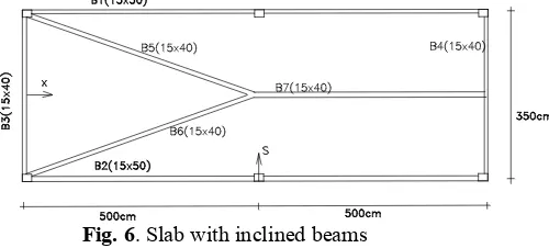
The next example is the slab with beams inclined with respect to their edges shown in Figure 6. Loading data, supports and dimensions are the same as the previous example.
Fig. 6. Slab with inclined beams
[image:4.595.319.557.98.471.2] [image:4.595.323.564.102.250.2] [image:4.595.318.550.310.448.2] [image:4.595.60.299.328.429.2] [image:4.595.308.558.549.662.2]0 0.2 0.4 0.6 0.8
0 200 400 600
S(cm)
w(
cm
) BEM
[image:5.595.63.286.65.201.2]FEM
Fig. 7. Vertical displacement along beam B6 Figure 8 show the vertical displacement along beam B7 and Figure 9 show the results along coordinate s. These results show an excellent concordance among BEM a FEM analysis.
0 0.1 0.2 0.3 0.4 0.5 0.6 0.7 0.8
0 200 400 600
S2
w(
cm
)
BEM FEM
[image:5.595.320.545.83.300.2]Fig. 8. Vertical displacement along beam B6
0 0.2 0.4 0.6 0.8
0 100 200 300 400
S3
W(cm)
[image:5.595.62.286.314.455.2]BEM FEM
Fig. 9. Vertical displacement along S2
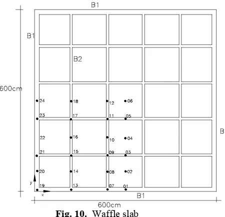
Te next example is a waffle slab supported at the four corners, as presented in figure 9. The plate has a constant thickness of 5 cm, and is subjected to a uniform load of 7.5kN / m². The boundary beams (B1) cross section is 20cmx60cm and the internal beams (B2) cross section is 8cmx40cm. In the numerical analysis the concrete data
assumed are: Young's modulus E = 2380kN/cm2 and
Poisson's ratio = 0.2.
Fig. 10. Waffle slab
Table 1 shows the results obtained in the analysis of this slab with the proposed formulation and those obtained with finite element method. For the BEM analysis a mesh with 40 boundary elements, 60 beam elements and 100 nodes were used. For the FEM analysis were adopted two meshes, one of 400 and another of 1600 finite elements. These results show excellent agreement among both formulations.
TABLE I
WAFFLE SLAB ANALYSIS RESULTS nodes Coordinates Displacements w(cm)
x y BEM FEM 400 FEM 1600
1 300 0 0.2682 0.26478 0.26815
2 300 60 0.5416 0.54084 0.54159 3 300 120 0.7674 0.76508 0.76684 4 300 180 0.9565 0.95421 0.95607 5 300 240 1.0640 1.0610 1.0636 6 300 300 1.1111 1.1079 1.1102
7 240 0 0.2554 0.25513 0.25528
8 240 60 0.5118 0.51039 0.5114 9 240 120 0.7389 0.73663 0.73832 10 240 180 0.9153 0.91237 0.91455 11 240 240 1.0260 1.0231 1.0256 12 240 300 1.0640 1.0610 1.0636
13 120 0 0.1585 0.1584 0.15849
[image:5.595.307.538.441.780.2] [image:5.595.74.287.538.660.2]18 120 300 0.7674 0.76508 0.76684
19 0 0 0 0 0
20 0 60 0.08351 0.08342 0.08347
21 0 120 0.1586 0.1584 0.15849
22 0 180 0.2176 0.21737 0.21749 23 0 240 0.2554 0.25513 0.25528
24 0 300 0.2683 0.268 0.26815
VICONCLUSION
In this work practical examples of building floors are analyzed with a combination boundary element method, to represent the plate, with the solution of the differential equation of beams to represent the interaction tractions among these two structural elements. Adopting a linear distribution for the traction between plate and beam the solution of the differential equation is a fifth degree polynomial which is then written as a function of the nodal parameters adopted for the beam. So the integral equations for the plate are written exclusively in function of the nodal displacements of the boundary of the plate and beams. The results were compared with those of the finite element method showing excellent agreement.
REFERENCES
[1] BÉZINE, G. A boundary integral equation method for plate flexure with conditions inside the domain. Int. J. for Numerical Methods in Engineering, 17: 1647-1657, 1981.
[2] PAIVA, J.B.; VENTURINI, W.S. Boundary element algorithm for building floor slab analysis. Boundary Element Technology Conference, Adelaide (Austr.) Nov., 1985.
[3] PAIVA, J.B.; VENTURINI, W.S. Analysis of building structures considering plate-beam-column interactions. International Conference on Boundary Element Technology- Rio de Janeiro- Jun., 1987.
[4] HARTLEY, G.A.; ABDEL-AKHER A.; CHEN P. Boundary element analysis of thin plates internally bounded by rigid patches. Int. J. for Numerical Methods in Engineering, 35: 1771-1785, 1992 [5] HU, C.; HARTLEY, G.A. Elastic analysis of thin plates with beam
supports. Engineering Analysis with Boundary Elements 13, p. 229– 238, 1994
[6] FERNANDES, G.R.; VENTURINI, W.S. Stiffened plate bending analysis by boundary element method. Computational Mechanics, 28, p. 275-281, 2002.
[7] FERNANDES, G.R.; VENTURINI, W.S. Building floor analysis by the boundary element method. Computational mechanics, 35, pp. 277-291, 2005.
[8] OLIVEIRA NETO, L.; PAIVA, J.B. A special BEM for elastostatic analysis of building floor slabs on columns. Computers & Structures, v.81, n.6, p.359-372, March, 2003. (ISSN: 0045-7949) [9] OLIVEIRA NETO, L.; PAIVA, J.B. Cubic approximation for the
transverse displacement in BEM for elastic plates analysis. Engineering Analysis with Boundary Elements, v.28, p.869-880, 2004. (ISSN: 0955-7997)
[10] KIRCHHOFF, G. Über das Gleichgewicht und die Bewegung einer elastichen Scheibe. J. Math., v.40, p.51-58, 1850.
[11] MENDONÇA, A. V.; PAIVA, J.B. Boundary Element Analysis of Plate-Beam Interaction. In: XXXII Jornadas Sud Americanas de Ingenieria Estructural, Santiago, 2008.
[12] PAIVA, J. B. ; MENDOÇA, A. V. A coupled boundary element/differential equation method formulation for plate beam interaction analysis. Engineering Analysis with Boundary Elements, v. 34, p. 456-462, 2010.
[13] Paiva, J.B. "Boundary element formulation for plate analysis with special distribution of reactions along the boundary". Advances in Engineering Software and Workstations 13: 162-168, July 1991 [14] M.N. De Rezende, J. Batista de Paiva, "A Quadrilateral Discrete
Kirchhoff Finite Element for Building Slab Analysis", in M. Papadrakakis, B.H.V. Topping, (Editors), "Advances in Finite Element Techniques", Civil-Comp Press, Edinburgh, UK, pp 25-31, 1994.