A Quantum Behaved Gravitational Search Algorithm

A Quantum Behaved Gravitational Search Algorithm

Mohadeseh Soleimanpour Moghadam, Hossein Nezamabadi-Pour, Malihe M. Farsangi

Electrical Engineering Department, Shahid Bahonar University of Kerman, Kerman, Iran Email: [email protected], [email protected], [email protected]

Received July 31, 2012; revised August 31, 2012; accepted September 15,2012

ABSTRACT

Gravitational search algorithm (GSA) is a recent introduced global convergence guaranteed algorithm. In this paper, a quantum-behaved gravitational search algorithm, namely called as QGSA, is proposed. In the proposed QGSA each individual mass moves in a Delta potential well in feasible search space with a center which is weighted average of all

kbests. The QGSA is tested on several benchmark functions and compared with the GSA. It is shown that the quan-tum-behaved gravitational search algorithm has faster convergence speed with good precision, and thus generating a better performance.

Keywords: GSA; Quantum Mechanics; kbest; QGSA

1. Introduction

The objective of global optimization is to find the glob- ally best solution of (possibly nonlinear) models, in the search space. Formally, global optimization seeks global solution of a constrained optimization model. Nonlinear models are ubiquitous in many applications, e.g., in ad- vanced engineering design, data analysis, financial plan- ning, scientific modeling, and others. These solutions of- ten require a global search approach.

The field of swarm intelligence is an emerging re- search area that presents features of self-organization and cooperation principles among group members bio-in- spired on social societies. Swarm Intelligence (SI) is the property of a system whereby the collective behaviours of agents interacting locally with their environment cause coherent functional global patterns to emerge.

Gravitational search algorithm (GSA), is a population based swarm optimization technique which was intro- duced by Rashedi et al. in 2009 [1], is a population based evolutionary optimization inspired by law of gravity. Similarly to genetic algorithms [2], GSA is an optimiza- tion tool based on a population, where each member is seen as a mass, and each mass is a potential solution to the problem under analysis. It has already been shown that GSA is comparable in performance with other evo- lutionary algorithms such as particle swarm optimization (PSO) [3] and Genetic Algorithm (GA) [2].

The basic idea of the GSA is to mimic the physical at- traction between masses. Agents are considered as ob- jects and their performance is measured by their masses. All these objects attract each other by the gravity force, and this force causes a global movement of all objects

towards the objects with heavier masses.

At the end of the 19th century, classical mechanics encountered major difficulties in describing motions of microscopic particles with extremely light masses and extremely high velocities, and the physical phenomena related to such motions. These aspects forced scientists to rethink the applicability of classical mechanics and lead to fundamental changes in their traditional understanding of the nature of motions of microscopic objects [4]. The studies of Bohr, de Broglie, Schrödinger, Heisenberg and Bohn in 1920s inspire the conception of a new area, the quantum mechanics [5].

Recently, the concepts of quantum mechanics and phy- sics have motivated the generation of optimization me- thods. Inspired by the GSA and quantum mechanics theories, this work presents a new Quantum-behaved GSA (QGSA) approach with outstanding result for uni- modal functions.

The rest of the paper is organized as follows: Section 2 describes the features of classical GSA for continuous optimization, while Sections 3 explains the QGSA. Sec- tion 4 presents the results of the optimization. Lastly, some conclusion remarks are given in Section 5.

2. Classical Gravitational Search Algorithm

movement of all objects towards the objects with heavier masses.

The procedure for implementing the classical version of GSA is given by the following steps:

Step 1. Initialization of agent positions: Initialize a population (array) of agents with random positions in the D-dimensional problem space using uniform probability distribution function. To this aim, the GSA consider a system with agents (masses), the position of the th agent is defined as follows:

N i

1, 2, ,



1_{, ,} d_{, ,} n



_,

i i i i

X  x  x  x i  N

d

(1)

where x_i is the position of th mass in the th di-mension and is dimension of the search space.

i d



D

Step 2. Evaluation of agent’s fitness: Evaluate each agent’s fitness value.

Step 3. Update G t



, best

 

t , worst

 

t , M t_i

 



 

G G t



0,



 

 

 

 

for i1, 2, ,N: In GSA, the gravitational constant,

, will take an initial value, , and it will be reduced

by time: G G0

G t (2)

Based on [1], the mass of each agent is calculated after computing current population’s fitness as follows:

 

fit worst

best

i i

q t 

worst t t t t  

 

(3)

 

 

1 i s j j q t q t  





i

M t (4)

where M t_i



andfi_i





represent the mass and the fit-ness value of the agent at , and,

t t

i t worst

 

t and

 

bes

1, ,

 

max fit_j j s

t t

 

1, ,

 

min fitj j s

t t

 

i

t t are defined as follows (for a maximization problem):

 

best  (5)

 

worst  (6)

Step 4. Calculation of the total force in different direc- tions: The total forces from a set of heavier masses that apply on agent is calculated based on law of gravity as follow:

 

 

   

 



d

 

d

 



j i

best,

rand j i

d

i j

j k j i ij

M t M t

F t G t

R t 

 







x t x t

rand

(7) where j is a uniform random in the interval

 

0,1

 

,

ε is a small value, and R tij i

is the Euclidian distance between two agents and j defined as

 

 

 

₂

ij X ti , j .

R t  X t kbest is the set of first K

agents with the best fitness value and biggest mass.

best

k is a function of time, initialized to K0 at the be-

ginning and decreasing with time. Here, K0 is set to

(total number of agents) and is decreased linearly to 1.

N

 

Step 5. Calculation of acceleration and velocity: Agent acceleration is calculated by using law of motion as fol- low:

 

 

 

 

 



 

 



best, rand d i d i i

j d d

j j i

j k j i ij

F t a t

M t

M t

G t x t x t

R t 

     



rand (8)

 

where i is a uniform random in the interval 0,1 . Then, the next velocity of an agent is calculated as a fraction of its current velocity added to its acceleration.



1



rand

 

 

d d d

i i i i

v t  v t a t

i

(9) Step 6. Updating agents’ position: Change the agent’s position, x , according to Equation (10).



1



 



1



d d d

i i i

x t x t v t (10) Step 7. Repeating the evolutionary cycle: Repeat steps 2 to 6 until the stop criteria is reached, usually a suffi- ciently good fitness or a maximum number of iterations (generations).

3. Quantum Formulation of the Agent

Dynamics

As per classical mechanics, an individual is depicted by its position vector xi and velocity vector i, which determine the trajectory of the individual. The individual moves along a determined trajectory in Newtonian me- chanics, but this is not the case in quantum mechanics. In quantum world, the term trajectory is meaningless, be- cause i

v

x and i of an individual cannot be determined simultaneously according to uncertainty principle. There- fore, if individual agent in a GSA system has quantum behavior, the GSA algorithm is bound to work in a dif- ferent fashion.

v

In quantum time-space framework, the quantum state of an individual is depicted by wave function

 

 in- stead of position. is the probability that measurement of the individual’s position finds it about the point whereby

Q

2 Q

  .

In quantum mechanics, the governing equation is the general time-dependent Schrödinger equation,

 

,

   

,

j r t H r r t

t 

 _



 (11)

 

where H r

 

is a time-independent Hamiltonian opera- tor given by,

 

2 2

2

r V r

m

    

where is Planck’s constant,mis the mass of the indi-vidual, and is the potential energy distribution. Its amplitude squared is the probability that measurement of the individual’s position at the time finds it in the volume element about the desired point. By imposing the following normalization condition we can justify such a measure,





V r

t



2 







dr Q rd 1











 

(13)

Now, we hypothesize that the GSA system is a quan-tum system, each mass of which is of quanquan-tum state for-mulated by wave function. Inspired by analysis of con-vergence of the classical GSA in [1],we assume that an individual mass moves in a Delta potential well in feasi-ble search space, of which the center is weighted average of all kbest. For simplicity, we consider an agent in one-dimensional space, the potential energy of the mass in one-dimensional Delta potential well is represented as:

 

V r   r (14)

where  is a positive number proportional to the “depth” of the potential well. The depth is infinite at the origin and zero elsewhere.

The Schrodinger equation for the model is,

 

 

   

r  r

 

0

r

2 2

2

E r

m

  _    (15)

For the equation can be written as,

2

dr 

2 2

d _2m_{E 0}

 (16)

In order to prevent diverging of agents the following boundary conditions is applied

0



   

r (17)

To satisfy the bound condition, Equation (16) is cal-culated as follow:

 

2mEr r

 _e  _{when r}₀

rand

 

 

(18)

QGSA is the integration of quantum computing and GSA. The QGSA is based on the representation of the quantum state vector.

To evaluate the fitness value, we need to learnof pre-cise information of position of the agent. However, the quantum wave function can only give the probability density function that the mass appears at the desired position. Sowe have to gauge the position of the indi-vidual, which is called collapsing the quantum state to the classical state. According to Monte Carlo Method of uncertainty, it is possible to simulate the process of measurement. The procedure of simulation is described

as follows.

To this aim, a random variable is generated un- iformly distributed between 0 and 1, so Equation (18) can be simplified with substituting a random number instead of it,

2 2 2

e rand

mE r Q r  r



   

rand

(19)

where is a random number uniformly distributed on

 

0,1 .





best ln rand 2 2

r x

mE

   





(20)

Thus, the position of agent accurately is measured as follows,





best ln rand 2 2

x

mE

 





(21)

where

2 2mE 

is the only parameter of the algorithm.

The procedure for implementing the QGSA is given by the following steps:

Step 1. Initialization of mass positions: Initialize a population (array) of masses with random positions in the D-dimensional problem space using a uniform prob-ability distribution function.

Step 2. Evaluation of particle’s fitness: Evaluate the fitness value of each agent.

Step 3. Selecting kbest and update Pbest: kbest is the set of first Kagents with the best fitness value and biggest mass. In order to updating Pbest, compare each agent’s fitness with the agent’s Pbest. If the current value is better than Pbest, then set the Pbest value equal to the current value and the Pbest location equal to the cur- rent location in D-dimensional space.

Step 4: Updating the Mbesti using Equation (23):

,

distance_{i l}  X_ikbest_l (22)

1

,

1

,

1 _best

distance best

1 distance

K j

i j i

K l

i l k M













c

[0,1]

j

(23)

Step 5. Updating of masses’ position: Change the po-sition of the mass where c₁ and ₂ are two random numbers generated using a uniform probability distribu-tion in the range .

1 2

1 2

best best

Best

d d

d _{i i}

i

c M c P

c c

 

 (24)





 





 

1

1 Best Best ln

rand 1

1 Best Best ln

rand

i i i i

i i i i

X t X t

X t X t

   _{     }    _{     }  if 0.5 if 0.5 S S   _       _     (25) where  is a design parameter called contraction-ex- pansion coefficient, and are values generated according to a uniform probability distribution in range

rand S

 

0,1

D

.

Step 6. Repeating the evolutionary cycle: Loop to Step 2 until a stop criterion is met, usually a sufficiently good fitness or a maximum number of iterations (generations).

4. Numerical Results

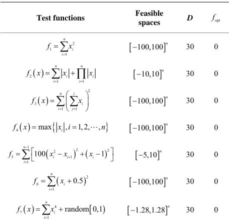
In this study, to evaluate the performance of the QGSA, 7 minimization benchmark functions [1,4] listed in Table 1 are used for comparison with classical GSA. In Table 1,

is the dimension of search space (function), fopt is

the minimum value of the function. The minimum value (fopt) of the functions of Table 1 are zero. The test

func-tions are unimodal high-dimensional funcfunc-tions which make them suitable for evaluating performance of the algorithm in point of view convergence rate.

We evaluate the unimodal optimization algorithm in two aspects: quality, and precision of solutions.

Quantity: Number of needed fitness function evalua-tions to reach the global optimum. It means the conver-gence rate of search algorithm.

[image:4.595.308.539.133.500.2]

Precision or accuracy: The difference between the glo- bal minimum and one but lowest minimum determines the possibility to detect the global minimum point.

Table 1. Benchmark functions used in this study.

Test functions Feasible

spaces D

Table 2. Minimization result of functions in table 1. Results are averaged over 30 runs and the average best-so-far and standard deviation of best solution obtained at last iteration are given.

Classical

GSA Quantum GSA

The average best-so-far solution

median of the best solution the standard deviation

7.3e−11 7.1e−11 4.4e−25

0 0 0 1 f The average best-so-far solution

median of the best solution the standard deviation

4.03e−5 4.07e−5 1.38e−013

0 0 0 f₂ The average best-so-far solution

median of the best solution the standard deviation

0.16e+3 0.15e+3 1.05e+4 0 0 0 f3 The average best-so-far solution

median of the best solution the standard deviation

3.7e−6 3.7e−6 1.4e−4

0 0 0 f4 The average best-so-far solution

median of the best solution the standard deviation

25.27 25.17 181.83 1.112 0 33.156 f5 The average best-so-far solution

median of the best solution the standard deviation

8.3e−11 7.7e−11 2.41e−32

1.176e−3 0 7.87e−3

f6

The average best-so-far solution

median of the best solution the standard deviation

0.018 0.015 1.02e−4

0 0 0 f7 opt f 2 i 1 1 n i f x 





_ 100,100_n

 30 0

  2

In unimodal functions, the convergence rate of search algorithm is more important than the final results because there are other methods which are specifically designed to optimize unimodal functions.

1 1

n n

i i

i i

f x x x

 









_ 10,10_n

   30 0 2 1 1 n i i i j 3

f x x

 

 

 

 

 

 _ 100,100_n

 30 0

 





4 max i, 1, 2, ,

f x x n  100,100n



 i i

 _ 

  5,10n

6 1 n i i f x 





 _100,100_n

4 _r

i x

  _ 1.28,1.28_n

 i

   30 0

 

2 2 1 i 1

x  x

1 2 5 1 100 n i

f  x







 30 0

 2

0.5 30 0

  7 1 n i f x 



andom 0,1  30 0

The results are averaged over 30 runs and the average best-so-far solution, median of the best solution and the standard deviation in the last iteration are reported for unimodal functions in Table 2. As this table illustrates

QGSA provides better results than GSA for all functions. In these function QGSA tends to find the global optimum faster than classical GSA and hence has a higher con-vergence rate.

The numerical results in Table 2 show that almost the

QGSA could hit the optimal solution with high precision. There are two exception test functions which QGSA cannot tune itself and have not a good performance.

[image:4.595.57.286.508.732.2]

valley is trivial, so converging to the global minimum, however, is difficult. Hence QGSA could not tune itself.

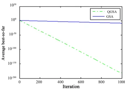
Also, the good convergence rate of QGSA could be concluded from Figures 1 to 7. According to these

[image:5.595.314.528.86.238.2] [image:5.595.318.529.289.441.2]

fig-ures, QGSA tends to find the global optimum in an ac-ceptable time hence has a high convergence rate.

[image:5.595.62.282.363.514.2]

Figure 1. Comparison of performance of QGSA and GSA for minimization of f1

 

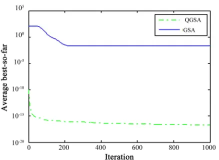
x .

Figure 2. Comparison of performance of QGSA and GSA for minimization of f2

 

x .

Figure 3. Comparison of performance of QGSA and GSA for minimization of

[image:5.595.316.531.491.639.2]

Figure 4. Comparison of performance of QGSA and GSA for minimization of f₄

 

x .

Figure 5. Comparison of performance of QGSA and GSA for minimization of f₅

 

x .

Figure 6. Comparison of performance of QGSA and GSA for minimization of f6

 

x .

The reported results for dimension 30 by for different test functions are summarized in Table 2. According to Figures 1 to 7, we can see that QGSA provides better

solutions except for

 

3 x . ₆

 

[image:5.595.71.280.565.702.2]

[image:6.595.63.282.84.244.2]

Figure 7. Comparison of performance of QGSA and GSA for minimization of f₇

 

x .

5. Conclusion

In this paper, a quantum version of gravitational search algorithm is introduced called as QGSA. It is tasted on different benchmark functions to investigate the effi- ciency of QGSA. The results show that QGSA is per- forming much better than GSA in finding the optimum result. Although the used functions are unimodal func- tions but it could expand it to multimodal functions. Currently, the authors are working on the improvement

of the proposed QGSA.

REFERENCES

[1] E. Rashedi, H. Nezamabadi-Pour and S. Saryazdi, “GSA: A Gravitational Search Algorithm,” Information Science, Vol. 179, No. 13, 2009, pp. 2232-2248.

doi:10.1016/j.ins.2009.03.004

[2] K. S. Tang, K. F. Man, S. Kwong and Q. He, “Genetic Algorithms and Their Applications,” IEEE Signal Proc-essing Magazine, Vol. 13, No. 6, 1996, pp. 22-37 doi:10.1109/79.543973

[3] F. V. D. Bergh and A. P. Engelbrecht, “A Study of Parti-cle Swarm Optimization PartiParti-cle Trajectories,” Informa-tion Sciences, Vol. 176, No. 8, 2006, pp. 937-971. doi:10.1016/j.ins.2005.02.003

[4] X. F. Pang, “Quantum Mechanics in Nonlinear Systems,” World Scientific Publishing Company, River Edge, 2005. doi:10.1142/9789812567789

[5] W. Schweizer, “Numerical Quantum Dynamics,” Hing- ham, 2001.