Bayesian Prediction of Bi Component State Space Model to Chinese Population

2019 International Conference on Computer Intelligent Systems and Network Remote Control (CISNRC 2019) ISBN: 978-1-60595-651-0

Bayesian Prediction of Bi-Component State Space

Model to Chinese Population

Shuaipeng Li and Weibo Hou

ABSTRACT

A series of problems brought by the growth of population are perplexing all over the world with the accelerating process of globalization. Therefore, it is urgent to study population prediction, and use the cohort component method and bi-component state space model for predicting population reasonably and effectively, thereby reducing resource waste, and adhering to the path of sustainable development.

KEYWORDS

Bayesian Prediction, Cohort Component Method, Bi-component State Space Model.

INTRODUCTION

Chinese population has accounted for a large proportion of the world population since ancient times. The important policy of family planning has been made bythe Central Committee of the Communist Party of China early in 1962. The fertility rate was declined continuously under the population replacement rate with continuous strengthening of family planning work in 1890s. Although the population is increasing every year, the proportion in world total population is decreasing and the aging degree is increasing year by year due to the population structure. , Chinese population has reached 1.39538 billion (excluding Hong Kong, Macao, Taiwan and overseas Chinese) at present, wherein 713.51 million are men and 681.87 million are women, men are far more men than women, and the sex ratio of the total population is 104.64. The problem of population aging is becoming more and more serious although the population is large in terms of numbers, total population aged 65 or above is 166.58 million, accounting for 11.9% of total population. Even so, the fertility rate is still decreasing. The total fertility rate is 10.94‰ (the fertility rate per 1,000 women). However. the future population is still unknown with the release of the second child policy.

United Nations and the World Bank prepared global and national population prediction for all countries, thereby laying a foundation for sustainable development of the world. The requirements on food, water, energy and other natural resources and even the prediction to commercial and industrial scale can be mastered as far as possible in the future. Therefore, the policy planning and formulation in the aspects of

_________________________________________

Shuaipeng Li, Weibo Hou

economy, health care, social security, education, infrastructure, tax expenditure, etc. are closely related to population.

Many experts and scholars at home and abroad studied population prediction. Stefan McKinnon, Edwards, Jaap B. Buntjer, etc. used group design for accurate prediction[1], Hossein Vahidi Monfared and Alireza Moini developed prediction system dynamics model of Iranian population[2]. Cui Xiaodong analyzed the nursing needs of elderly population in China based on multi-state Markov[3]. Meng Xiangjing and Jiang Kaidi made an in-depth study on the age structure of urban and rural population in China in the future based on the urbanization policy[4]. Jia Hongwen et al. took Gansu Province as an example to explore population prediction and development trend[5].

COHORT COMPONENT METHOD

The cohort component method was firstly proposed by Whelpton in 1936, which was refined by Lesile in 1945 aiming at studying factors affecting population fluctuations. The cohort was divided according to age and gender groups, and the components were birth rate, mortality rate and migration, which were obviously three processes leading to population change. Meanwhile, the cohort component method can be applied for predicting the population, population scale and composition of each age gender subgroup (age distribution). The key statistics are shown as follows:

The mortality rate divided according to age groups within one year=age group deaths calculated according to year/the age group calculated according to mid-year population scale:

The fertility rate divided according to age groups within one year= delivery of women in the same age group within one year /mid-year population scale of women at the age.

The total fertility rate also belongs to indispensable key data in addition to the above-mentioned mortality rate and fertility rate, namely the total number of children produced by one woman in her lifetime, namely the current age specific fertility rate thereof. Next, the relevant equation of population change factor synthesis is introduced as follows[6]:                                                              M t F t M t F t M t M t F t F t M t F t I I P P s b s b P P 0 0 0 0 1 1

The population is divided according to age groups when the gender is k. The mid-year population scale at the t mid-year is shown as follows:

P0,, ,P85,,k M(male)orF(female)

P k t k t k t     

86 age groups are formed here:

) 85 ( 85 84 1

The birth rate of female age group at the t year with gender k is shown as follows:

 

0,, 14,,, 45,,0,,0 k

t k

t k

t b b

b

The conditional survival rate of the age group at the t year with gender k is shown as follows:                  k t k t k t k t k t k t s s s s s s , 85 , 84 , 83 , 1 , 0 0 0 0 0 0 0 0 0 0 0 0 0         

The net immigration population in the age group at the t year with gender k is shown as follows:





I k t k t k t     _ Here:

 x t F t x t x F t F t

x f s f

m a

b , , 1,

, 0 , 2 1 5 . 0

1    

  

_

_

x f s f

m a

b , , 1,

, 0 , 2 1 5 . 0 1 1        k t x k t x k t x m m s , , 1 , 5 . 0 1 5 . 0 1      

Wherein, a 11maleandfemalebirthratio _{refers to the proportion of baby girls,} fx,t _refers

to the fertility rate of x years old at t year, and

k t x

m _,

refers to themortality rate of x years old with gender k at t year.

Population prediction is a high, middle and low prediction based on the mortality rate, fertility rate and population migration. It can be directly evaluated by probability prediction instead of deterministic prediction. Bayesian method is a systematic and natural method, wherein all known sources of uncertainty are included into the prediction. The mortality rate, fertility rate, and population migration prediction are introduced as follows.

MORTALITY RATE PREDICTION

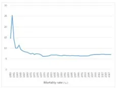
The mortality rate has been decreasing over the past 40 years as an important influencing factor of population prediction. The mortality rate prediction model: Lee-Cater model is introduced here:

t x t x x t

x a b K

m_{, ,}

Wherein, ax _{denotes the general age pattern of death (determined with time),}

t

K

denotes the general morality rate profile with time, bx_{denotes the} Kt_{coefficient of}

different age groups, x,t~independentdistribution_,

 

2

, 0 _x

N  _.

Figure 1. Data of Chinese historical mortality rate.

t

K _{refers to random change with constant movement.}

t t

t K

K  1

ion tdistribut independen

t ~



, N

 



n

t Kt _,

1 1 



G

x bx . Parameters are estimated according to historical data in Figure 1.

Parameters and Kt_{grades can be predicated according to estimation aiming at future}

mortality rate.

The lee-carter model is very suitable for the mortality rate trend in many countries. However, it has few parameters. Although it is the most widely used model in the mortality rate prediction, the age-time interaction is not considered, and the prediction error is underestimated. Therefore, we should optimize the bayesian method in the model and get the bayesian method of Lee-Carter Model[7].

Parameter

2 2

, ), , , 1 ( , , ), , , 1

(t n a b  x G 

Kt   x x x   _{is obtained through their}

combined posterior distribution, and the priors are given by non-informational prior distribution. MCMC method is adopted in order to extract a sample from the combined posterior distribution. In the method, iterative sampling is achieved through the conditional distribution of each parameter assigned to all other given parameters.

The Kt(t1,,n)_{status is predicted and updated by Kalman filter, and it is sampled}

smoothly by Kalman in MCMC.

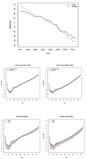
Data from 1975 to 2006 is used as training samples during in-sample prediction. Data from 2007 to 2012 is used as test samples. Then, out-of-sample prediction of 2018-2034 is performed based on the fitted data from 1975 to 2012. The convergence is tested by the trace map and Gelman-Rubin statistics by using non-information priors of model parameters. The initial value is scattered, which is iterated for 2000 times.

The posterior distribution of 3000 sample parameters is predicted in MCMC based

on Lee-Carter model[8], the Kt _{state is predicted. They are stratified according to}

Figure 2. Mortality rate estimation state Kt_.

TABLE III. Expected life prediction during birth (year). 2018 2034

Male 98.1% 78.4 88.6 mean 77.5 84.9 1.9% 76.5 81.7 Female 98.1% 83.9 89.6 mean 81.4 85.5 1.9% 77.7 79.8

It can be seen from TABLE III that the life span of both men and women at birth has been increased with time, which is closely related to social factors such as human increasing living standard, medical environment, etc.

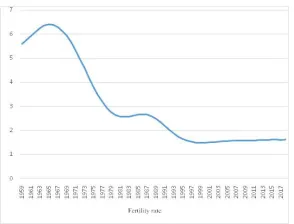
FERTILITY RATE PREDICTION

Figure 3. Fertility rate change with time.

The fertility rate prediction model: bi-component state space model is introduced as follows:

t x t x t x x t

x r

f _{, ,}

ln      

In the above formula, x _{represents a general age model of fertility (unchanged}

with time), t _{represents the linear trend with time,} t _{represents non-linear trend}

with time, x,rx _{refers to age-specific slope coefficient about} t,t_, ion

tdistribut independen

t x, ~ 

,





2

0 Vx

N ， _.

Wherein the linear time trend of the bi-component state space is shown as follows:

t t

t  

 _1

ion tdistribut independen

t~

 _,





0，

N _{; nonlinear time trend is shown as follows:}

t t

t   

  _1 

ion tdistribut independen

t ~

 _{, N}





. t,t _{are orthogonal:}



  

n

t t t

1

0



Wherein, constraint conditions include the follows:









t t x x

x x

t

t 0,  0,  1, r 1

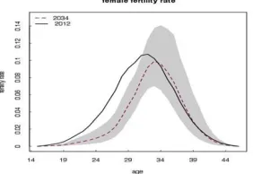
Figure 4. Process estimation of two potential components.

Figure 5. In-sample prediction: 2012.

Figure 6. In-sample prediction: 2007-2012.

POPULATION MIGRATION PREDICTION

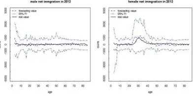
Figure 8 shows that Chinese migration data is not accurate and stable enough so the number of net migration in each age-gender-time group is obtained indirectly from population and mortality rate data. The net migration scale of each age group is the result based on the single-vector state space model similar to Lee-Carter model. Bayesian prediction (size of 3000) of model parameters are sampled from MCMC posterior distribution.

Figure 8. Historical migration data in China.

Figure 9. Net migration sample prediction: 2012.

BAYESIAN POPULATION PREDICTION

Population change factor formula is used based on Bayesian prediction on mortality rate, fertility rate and migration, here:





1  

babygirlratioatbirth

a

Wherein, 1.18 represents the average gender ratio in China from 2010 to 2014 at birth (M:F). The global historical average gender ratio at birth is higher than 1.05. 2006 in-sample prediction population or 2012 out-of-sample prediction population is regarded as the baseline population, the probability of obtaining the prediction result from the bayesian process (MCMC sample) natural is 95% as shown in Figure 9.

prediction and in-sample prediction are carried out according to the known historical data, and the processing results are shown in the following figure[9].

TABLE IV. Deviation degree of Chinese population (10,000 people) sampling prediction (posterior mean - real number).

2007 2008 2009 2010 2011 2012

Male 98.1% 68048 68357 68647 68748 69068 69395 mean 68048 68244 68451 68673 68886 69006 1.9% 68032 68047 68321 68420 68791 68897

bias 7 15 23 37 46 36

Female 98.1% 64081 64445 64803 65343 65667 66009 mean 64002 64374 64533 65214 65539 65586 1.9% 63998 64256 64403 65013 65475 65499

bias -5 -6 -14 -17 -14 -25

Total 98.1% 132129 132802 133450 134091 134735 135404 mean 132919 133007 133088 133161 133225 133281 1.9% 132902 132975 133036 133082 133113 133134

bias 2 9 9 20 32 11

Figure 10. Chinese population sampling prediction: male (ten thousand people).

Figure 12. Chinese population sampling prediction: total.

Figure 13. Age condition of observation and in-sample prediction (2012).

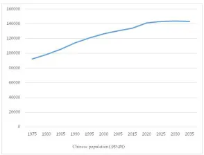
Figure 14. Chinese population prediction: 2018-2034.

MAIN CONCLUSIONS

The Lee-Carter model is in good agreement with Chinese mortality rate data, and accurate in-sample prediction is provided;

The newly proposed two-component state space model with orthogonal linear and nonlinear trend components is fitted well to China fertility rate data;

REFERENCES

1. Stefan McJinnon Edwards, Jaap B. Buntjer, Robert Jackson. The effects of training population design on genomic prediction accuracy in wheat[J].Theoretical and Applied Genetics, 2019, 132(07):1943-1952.

2. Hossein Vahidi Monfared, Alireza Moini. A system dynamics model to prediction the population aging in Iran[J].Kybernetes, 2019, 213(04):1216-1241.

3. Cui Xiaodong. Prediction of long-term care needs of elderly population in China—based on multi-state segmental constant Markov analysis. Chinese Population Science, 2017, 32(06):82-93.

4. Meng Xiangjing, Jiang Kaidi. Influence of urbanization and rural-city transfer on the age structure of urban and rural population in China in the future. Population Research, 2008, 42(02):39-53.

5. Jia Hongwen, Xie Zhuojun, Gao Yigong, Prediction and development trend analysis of population in Gansu Province. Population of Northwest China, 2008, 39(03):118-126.

6. Shi Renbing, Chen Ning. Test of results of Chinese population prediction and comparison of influencing factors. Statistics and Decision-making, 2008, 67(17):14-18.

7. He Xiaolin. Establishment and application of multi-factor population prediction model based on age shift algorithm. Statistics and Decision-making, 2008, 67(21):23-26.

8. Su Yaling, He Youhua. Bayesian estimation of non-parametric regression. Journal of Shanghai University (natural science edition), 2008, 24(06):1022-1029.