2016 Joint International Conference on Artificial Intelligence and Computer Engineering (AICE 2016) and International Conference on Network and Communication Security (NCS 2016)
ISBN: 978-1-60595-362-5
A Modified Algorithm for a Density-based Clustering Method
Ze-Lu Deng
1,2,a, Jian-Bin Gao
1,2,b,*, Qi Xia
2,3,c1School of Resources and Environment, University of Electronic Science and Technology of China, Chengdu, Sichuan, China
2Center for Big Data, University of Electronic Science and Technology of China, Chengdu, Sichuan, China
3School of Computer Science and Engineering, University of Electronic Science and Technology of China, Chengdu, Sichuan, China
a[email protected], b[email protected], c[email protected]
*Corresponding author
Keywords: Gray Image Segmentation, Clustering Method, Fast Algorithm.
Abstract. We develop a fast algorithm for a density-based clustering method [1] when it is applied to gray image segmentation. To achieve this, we rely on the property that a gray image has no more than 256 gray levels. This will help us reduce the computing time by a factor of 300 while still keep the performance.
Introduction
Clustering is to segment the physical or abstract collection of objects into different groups, making that the objects in the same group have a relatively higher similarity and vice versa. There are so many clustering methods such as K-Means [2], DBSCAN (Density-Based Spatial Clustering of Applications with Noise) [3], DIANA (Divisive Analysis) [4] and so on. Also in computer vision, clustering is a very important unsupervised learning method and widely used in image processing tasks, e.g., image segmentation. For example, in the work [5] by P. Hannequin et al, they propose an automatic algorithm to select regions of interest which is based on factor analysis and clustering analysis. In the work [6] by P. Arbelaez et al and the work [7] by M. Donoser et al, they finally use a hierarchical clustering method on an over-segmentation image to get the results. Recently, in the work [8] by Jian Hou et al, they propose a parameter-free algorithm based on the DSets (dominant sets) and DBSCAN algorithms. In this paper, we will first present a density-based clustering method [1] and analyze its shortcoming, then we’ll introduce our optimization strategy when this method is applied to gray image segmentation. Finally, in the experiment section, we will compare our method with the original algorithm in time consumption, and we can see that our method reduces the computing time by a factor of 300.
Original Algorithm
In the work [1], A. Rodriguez et al introduce a density-based clustering method of which the input is a distance matrix d and a radius r. The distance matrix d stores the distance of two data points and here the distance is equal to the dissimilarity between them. The radius r is a parameter set manually. For each data point, we need to compute three parameters. The first parameter is the local density ρ and for each data point i ρi is defined as:
ρi = ( ij )
j
d r
Here the dij is an element of distance matrix d and it represents the distance between data point i
and data point j. The parameter r is a cutoff distance. Besides
( )x = 1 if x < 0 and
( )x = 0 otherwise. Basically, ρi is equal to the number of data points that are closer than r to data point i. The second one we need to compute is the parameter δ and for each data point i δi is measured by computing theminimum distance between the point i and any other point with a higher density. It can be formulated as:
δi =min ( ):
j i ij
j d . (2)
And for the data point k with the highest density, they take δk = max(δ). As for the third parameter
n, for the data point ini is number of data point j, namely ni = j, which has a higher density and the
minimum distance dij at the same time. The parameter n can be seen as a by-product when computing
the parameter δ. The core of this algorithm is the parameter ρ and δ by which they can find out the right number of the clusters and the cluster centers and then they use the parameter n to assign every data point to a corresponding cluster. For more details about this algorithm, you can see in [1].
The shortcoming of this algorithm is very obvious. If our input is not a distance matrix, instead, it’s a gray image or more generally, the input are some data points with each described by a n-dimension vector, then we have to compute the distance matrix and that’s the problem. It takes a very long time to compute the distance matrix and if the data points are too large, we also need a large memory to store the distance matrix. The latter problem is very common in image processing, for example, given a 100×100 image, we assume that it takes 4 bytes to store an element of distance matrix and it comes out that we need about 0.37GB to store the distance matrix. In next section, we will show our approach to solve the problems above when this algorithm is applied to gray image segmentation.
Optimization Strategy
When algorithm mentioned above is applied to gray image segmentation, we can reduce time dramatically based on the gray image’s property that a gray image has no more than 256 gray levels. In the following part we will introduce optimization strategy.
First of all, we divide the original algorithm into two parts. The first part is to compute the local density ρ and the second part is to compute parameters δ and n. What’s more, we don’t need a large memory to store the distance information. Then we also divide our optimization strategy into two parts. The first part is to reduce time of computing ρ and the second part is to reduce time of computing δ and n.
In this paragraph, we will discuss our optimization strategy with regard to computing ρ. We find that for a gray image, the ρ of every pixel in the image is just related to its gray value. For example, given the radius r = 3, if we want to compute the ρ of a pixel with the gray value equal to 100. Then the ρi of this pixel can be written as:
ρi = num98,99,100,101,102. (3)
Here the num means the total number of a certain gray value in a given image. In Eq. 3, for instance, num98 means the total number of the gray value equal to 98 in the given gray image and it is not
difficult to understand that num98, 99,100,101,102 means the sum of num98, num99, …, num102. So from the
discussion above, we can find that the ρ of a pixel has nothing to do with the pixel’s location (x, y) in the image. Based on this idea, we use a 256×1 matrix Mρ to store the gray values and the
Mρ =
T
0 1 254 255
101 2
1 255 256
1000
x x x x
( ). (4)
But there are still two problems, one is that the different gray values may have the same total numbers and the other is that some gray values may not exist in a given gray image, in other words, their total numbers are equal to 0. The former may not seem important at this time, but we can’t go onto the second part unless we solve this problem. We adopt a very simple method to solve this, and the solution is that we add some small values such as 1, 2 to the total number to make sure that different gray values corresponds to different total numbers and vice versa. This operation will barely influence the final results. The latter problem will be solved naturally in the second part which we will present in the next paragraph. After getting the revised Mρ, we then can obtain the ρ for all pixels.
In this paragraph, we will discuss our optimization strategy with regard to computing δ and n. Let us review the definition of δ and n. For each data point i δi is measured by computing the minimum
distance between the point i and any other point with a higher density and ni is number of data point j
which has a higher density and the minimum distance dij at the same time. Actually the parameter n is
very easy to obtain when computing δ so we won’t talk much about it here. As we can see from the definition, there are two key points: higher density and minimum distance. The ρ we get in the first part for all pixels is actually N-dimension vector and here N is the total number of pixels in a given gray image. We first sort the ρ for all pixels in a descent order, as discussed above there are no than 256 different values of ρ. Then we use a 256×3 matrix Mδ to store the sorted vector. Mδ is defined as:
Mδ =
T
0 1 254 255
0 1 254 255
0 0 1 0 0 254 0 255
1 2 255 256
1 1 1 1 1
n
n
n n
p p p p p
N N N N N
N N N N N N N N N
.(5)
Here pn represents the n-th ρ, Nn is the number of pixels whose ρ is equal to pn and N0+N1+…+Nn+1
locates the next element in the sorted vector. Next we will give a simple example to show this. Supposing that we are given a 10-dimenson sorted vector as:
Vρ_ex =(7 7 7 7 4 4 4 2 2 1)T. (6)
Its Mδ can be written as:
Mδ_ex =
T
1 2 3 4 5 256
7 4 2 1 0 0
4 3 2 1 0 0
5 8 10 11 0 0
. (7)
If we detect that the location number exceeds the N, namely the dimension, we set other elements in this matrix to be zero. As shown in Eq. 7, we can see that 11>10, so other elements are set to be zero. In fact, this method also solves the problem we mentioned above. So what we do next is to use this matrix Mδ to obtain δ and n. As we revise Mρ in the previous paragraph, we are sure that the pixels
with the same value of ρ have the same gray value and this is what we base on. In the following discussion we will still take Eq. 6 and Eq. 7 as examples. When we use the definition to compute δ for every pixel in Vρ_ex (assuming that the gray values are known), we find that only the pixel at a sudden
change location has a positive value of δ, and the others are all zero. For example, the first 7, the first 4, the first 2 and the first 1. All of this are exactly what we record in the third column of the matrix Mδ.
The first 4 is the 5-th element in Vρ_ex and the first 2 is the 8-th element in Vρ_ex. The first element in
our algorithm. And the computation of the parameter n is almost the same. When we detect that the location number exceeds the dimension N, we will break our algorithm and move to the next part.
The previous two paragraphs have described the two parts of our optimization strategy. We will show in the experiment part that our algorithm reduces the computing time by a factor of 300 while still keeps the performance. And that’s our main contribution.
Experiment
The experiment is conducted on the computer with a quad-core and eight-thread CPU whose main frequency is 2.6 GHz and a memory of 16 GB. The algorithm is achieved on MATLAB R2016a. In all of our experiment, we set the parameter r = 4.
The main of the computing time of the original algorithm is spent on obtaining the distance matrix (if we have enough memory to store it), ρ and δ. Table 1 shows the time of computing distance matrix ρ, δ of a 200×200 gray image and the total time of getting the final results. The figures in the table are the average of the results of the ten experiments and in the table OA means original algorithm we mentioned above.
Table 1. Time consumption for a 200×200 gray image.
Part Time Consumption for OA (s) Time Consumption for Ours (s)
distance matrix 50.6742 0
ρ 64.4524 0.0085
δ 124.2862 0.0183
total 245.97 0.8083
The second column of Table 1 is the time consumption for the original algorithm and the third is for ours. In our algorithm, we don’t need distance matrix so the time consumption for it is 0. As we can see from the table, we reduce time of computing ρ by a factor of 7500 and δ by a factor of 6800 and the total time by a factor of 300.
In our other experiments, we find that if the gray image is a bit larger, such as a 256×256 one, MATLAB cannot store such a large distance matrix for this image. So we take the following strategy: we just compute the distances when we need them. But this strategy almost doubles the computing time in theory. Our algorithm is not very sensitive to the size of the gray image, as shown in Table 3 and Fig. 1. Table 2 shows the time consumption for a 500×500 gray image. The figures in the table are the average of the results of the ten experiments.
Table 2. Time consumption for a 500×500 gray image.
Part Time Consumption for OA (s) Time Consumption for Ours (s)
distance matrix 0 0
ρ 364.3642 0.0146
δ 577.3253 0.0434
total 953.6235 7.1188
Table 3. Time consumption.
Image Size Total Time Consumption (s) 100×100 0.8083
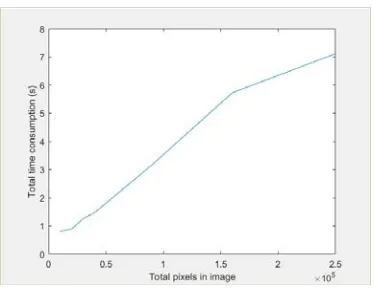
Figure 1. Total time consumption.
The reason why the time consumption for distance matrix of OA is 0 is that we adopt the strategy we stated in the previous paragraph. The rest elements in Table 2 are the same to those in Table 1. And Fig. 1 is just a line chart of Table 1, which is aims at giving us a more intuitive feeling about the influence of the growing image size on total time consumption.
Summary
In this paper, we do present a novel method to reduce the computing time for the algorithm we mentioned in the original algorithm section when it is applied to gray image segmentation, as we show in Table 1, we reduce the total computing time by a factor of 300. And we also find that our method is not very sensitive to the growing size of the gray image, as we illustrate in Fig. 1.
Acknowledgement
This work is supported in part by the Postdoctoral Science Foundation of China (2013M542267), Open Research Foundation of Integrated Electronic System of the Ministry of Education of China (20120105), the Fundamental Research Funds for the Central Universities (ZYGX2015J154), the applied basic research programs of Science and Technology Department (2015JY0043).
References
[1] A. Rodriguez, A. Laio, Clustering by fast search and find of density peaks, J. Science. 344 (2014) 1492-1496.
[2] J.A. Hartigan, M.A. Wong, A K-means Clustering Algorithm: Algorithm AS 136, J. Applied Statistics. 28 (1979) 100-108.
[3] M. Ester, H.P. Kriegel, J. Sander, X. Xu, A Density-Based Algorithm for Discovering Clusters in Large Spatial Databases, In Proceedings of the 2nd International Conference on Knowledge
Discovery and Data Mining, Portland, OR, 1996 pp. 226-231.
[4] R. Xu, D. Wunsch II, Survey of Clustering Algorithms, J. IEEE Transactions on Neural Networks, 16 (2005) 645-678.
[5] P. Hannequin, J.C. Liehn, J. Valeyre, Cluster Analysis for Automatic Image Segmentation in Dynamic Scintigraphies, J. Nuclear Medicine Communications. 11 (1990) 383-393.
[7] M. Donoser, D. Schmalstieg, Discrete-Continuous Gradient Orientation Estimation for Faster Image Segmentation, C. Conference on Computer Vision and Pattern Recognition (CVPR). (2014) 3158-3165.