Top-Down Selection in Convolutional Neural Networks

(1)

Top-Down Selection in

Convolutional Neural

Networks

Mahdi Biparva

A dissertation submitted to the Faculty of Graduate Studies

in partial fulfilment of the requirements

for the degree of

Doctor of Philosophy

Graduate Program in

Electrical Engineering and Computer Science

York University

Toronto, Ontario, Canada

September, 2019 c

(2)

Abstract

Feedforward information processing fills the role of hierarchical feature encod-ing, transformation, reduction, and abstraction in a bottom-up manner. This paradigm of information processing is sufficient for task requirements that are satisfied in the one-shot rapid traversal of sensory information through the visual hierarchy. However, some tasks demand higher-order information processing using short-term recurrent, long-range feedback, or other processes. The predictive, corrective, and modulatory information processing in top-down fashion complement the feedforward pass to fulfill many complex task require-ments. Convolutional neural networks have recently been successful in address-ing some aspects of the feedforward processaddress-ing. However, the role of top-down processing in such models has not yet been fully understood. We propose a top-down selection framework for convolutional neural networks to address the selective and modulatory nature of top-down processing in vision systems. We examine various aspects of the proposed model in different experimental set-tings such as object localization, object segmentation, task priming, compact neural representation, and contextual interference reduction. We test the hy-pothesis that the proposed approach is capable of accomplishing hierarchical

(3)

feature localization according to task cuing. Additionally, feature modulation using the proposed approach is tested for demanding tasks such as segmenta-tion and iterative parameter fine-tuning. Moreover, the top-down attensegmenta-tional traces are harnessed to enable a more compact neural representation. The experimental achievements support the practical complementary role of the top-down selection mechanisms to the bottom-up feature encoding routines.

(4)

Dedication

To my lovely wife, for her unconditional love and sacrifices ... To my mother, for her loving heart and prayers ...

To my father, for being so generous and considerate ... And to the one I am desperately seeking to visit one day ...

(5)

Acknowledgements

I am speechless to express how grateful I am to all the people who made this thesis possible. My sincere appreciation goes to my supervisor, Prof. John Tsotsos, whose knowledge and patience aided me considerably during my PhD journey. I am grateful to my supervisory committee, Prof. Richard Wildes and Prof. Marcus Brubaker, for their supports and insightful comments. I have been fortunate to be supervised by these wonderful people, and without them all, I could not have finished this thesis.

I am extremely grateful to all my close friends and colleagues who made this journey much more enjoyable and helped me through difficult times with their sincere supports and encouragement. My special thanks go to Calden Wloka, Markus Solbach, Toni Kunic, Mohammad Hosein Amini, Sajad Shirali-Shahreza, and Ali Mehrkish for their endless help and support during my PhD journey. My kind thanks go to all my previous teachers and instructors.

My deepest appreciation goes to my lovely wife, Najmeh Bordbar, who has always been next to me throughout the most difficult and challenging moments of my PhD program. Nothing I could ever do would repay you Najmeh for all sacrifices you have done for me. Without your love and support, this thesis

(6)

would not have happened.

I would like to express my eternally sincere gratitude to my father, Rasool, my mother, Zohreh, my sister, Zahra, and my brothers, Mohsen and Moham-mad Amin, who remotely far from home supported me throughout these years. I am also thankful to my father-in-law, Kamal, my mother-in-law, Zohreh, and my sister-in-law, Maedeh for their kind and sincere supports. I would be for-ever indebted for their unconditional love and encouragement. Thank you all for all the sacrifices you made to help me to complete this PhD.

Last but not least, I am grateful of the blessings that the God has bestowed upon me in this wonderful life, the opportunity to live long and healthy to see, think, and learn what, why, and how he has created in this amazing world.

(7)

List of Tables

3.1 Demonstration of the STNet configurations in terms of the hy-perparameter values. Lpropis the name of the layer at which the attention map is calculated. OF C and OBridge are the offset val-ues of the SI selection mode at the fully-connected and bridge layers respectively. αis the trade-off multiplier of the SC selec-tion mode. δpost represents the post-processing threshold value of the attention map. . . 63 3.2 Comparison of the STNet localization error rate on the

Ima-geNet validation set with the previous state-of-the-art results. The bounding box is predicted given the single center crop of the input images with the TD processing initialized by the ground truth category label. (1) Results calculated using the publicly published code by [1, 2]. (2) Based on the result reported by [2]. Otherwise, the results are reported by the reference work cited on the left. . . 64

(13)

5.1 The output channel size of computational units in the segmen-tation layers is given for AlexNet and VGG at three different levels. b, r, q are the units defined in 5.4.6. . . 127 5.2 Parallel and Sequential LSD performance results on the Pascal

VOC 2012 validation set once the BU network is fine-tuned on the extended Pascal dataset. . . 134 5.3 Comparison of different variants of SSN using AlexNet on

PAS-CAL VOC valid 2012. We use mean pixel accuracy and mean IoU metrics to report the performance. CAT, MAX, THD, ADD, and MUL stands for concatenation, top-1, and thresh-olding, additive, and multiplicative. . . 135 5.4 Comparison of SSN with the baseline model on PASCAL VOC

validation set using mean IoU metric. SSN++ is trained on the extended training set. . . 135 5.5 Comparison of SSN with the state-of-the-art on PASCAL VOC

2012 valid set. All methods use VGGNet as the backbone net-work. . . 135 5.6 Comparison of SSN with the baseline and state-of-the-art on

two additional segmentation benchmark datasets: CamVid and Horse-Cow. The results are reported on the test sets. Note that the DeepLab-LargeFOV* results are taken from[3]. . . 140 5.7 Ablation Studies on the TD modulatory role, the error

sig-nal propagation, number of gating layers into the segmentation pipeline using AlexNet on the Pascal VOC 2012 validation set. 146

(14)

6.1 LeNet error rate and compression ratio on MNIST dataset using the attentive connection pruning. . . 164 6.2 Comparison of the Compression ratio of the proposed method

with the baseline approaches using 300-100 and LeNet-5 network architectures on MNIST. Error degradation is the difference between the original error and the error at the end of the retraining phase. . . 165 6.3 LeNet and CifarNet error rate and compression ratio on

CIFAR-10 dataset using the attentive connection pruning. . . 168 7.1 The classification and localization rates of the selective

(15)

List of Figures

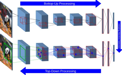
3.1 STNet consists of both BU and TD processing streams. In the BU stream, features are collectively extracted and transferred to the top of the hierarchy at which label prediction is generated. The TD processing (bottom), on the other hand, selectively activate part of the structure using attention processes. Fig-ure schematically illustrates AlexNet architectFig-ure. The middle blue boxes represent hidden and gating activity tensors on the BU and TD pathways. The last three squares represent fully-connected layers. Receptive fields are schematically depicted with small red boxes. The blue circles illustrate the selection regions that the information propagates to in the TD stream. . 56 3.2 Schematic Illustration of the sequence of interactions between

the BU and TD processing streams using the three-stage atten-tion process. . . 58

(16)

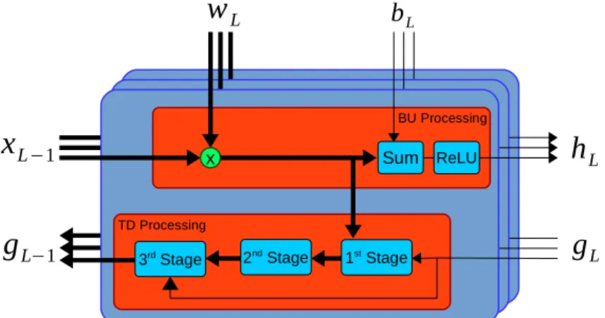
3.3 Modular diagram of the interactions between various blocks of processing in both the BU and TD streams. The arrow direc-tion shows the flow of the informadirec-tion to each computadirec-tional block. The layers schematically represent that the BU and TD processing is done on feature maps with spatial and channel dimensions. Thick arrows represent vector values while thin arrows represent scalar values . . . 59 3.4 Illustration of the predicted bounding boxes in comparison to

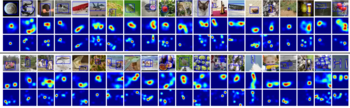
the ground truth for ImageNet images. In the top section, STNet is successful to localize the ground truth objects. The bottom section, on the other hand, demonstrates the failed cases. The top, middle, and bottom rows of each section de-pict the bounding boxes from the ground truth, ST-VGGNet, and ST-GoogleNet respectively. . . 65 3.5 Demonstration of the attention-driven class hypothesis maps for

ImageNet images. In both top and bottom sections, rows from top to bottom represent ground truth boxes on RGB images, the CH map from VGGNet, and the CH map from ST-GoogleNet respectively. . . 70

(17)

3.6 The critical role of the second stage of selection is illustrated using CH visualization. In the top row of each section, im-ages are presented with boxes for the ground truth (blue), full-STNet predictions (green), and second-stage-disabled predic-tions (red). In the second and third rows of each section, CH maps from the full and partly disabled STNet are given respec-tively. . . 72 3.7 We demonstrate using ST-VGGNet the confident region of the

accompanying object highly correlating with the true object category. The top row of each section contains images with the ground truth (blue) and predicted (red) boxes. CH maps highlight the most salient regions in the bottom row of each section. . . 73 4.1 Visual priming: something is hidden in plain sight in this image.

One is unlikely to notice it without a cue for what it is (for an observer that has not seen this image before). Once a cue is given, perception is modified to allow successful detection. See the supplementary material in Sec. A.2 for the full answer. . . 77 4.2 A neural network can be applied to an input in either an

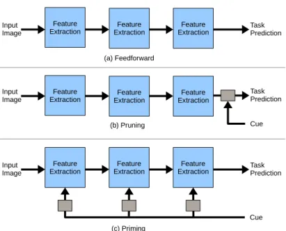
unmod-ified manner (top), pruning the results after running (middle) orpriming the network via an external signal (cue) in image to affect all layers of processing (bottom). . . 82

(18)

4.3 Overall view of the proposed method to prime deep neural net-works. A cue about some target in the image is given by an external source or some form of feedback. The process of prim-ing involves affectprim-ing each layer of computation of the network by modulating representations along the path. At the top, the stack of layers in N are schematically illustrated by the blue blocks. At the bottom, the coefficient parametersWi inNp are illustrated by the yellow blocks. . . 86 4.4 (a) Performance gains by priming different parts of the SSD

objects detector. Priming early parts of the network causes the most significant boost in performance. Black dashed line shows performance by pruning. (b) Testing variants of priming against increasing image noise. The benefits of priming become more apparent in difficult viewing conditions. The x axis indicates which block of the network was primed (1 for primed, 0 for not primed). . . 88 4.5 Effects of early priming: we show how mAP increases when we

allow priming to affect each layer in turn, from the very bottom of the network. Priming early layers has a more significant effect than doing so for deeper ones. The numbers indicate how many layers were primed from the first and second blocks of the SSD network, respectively. . . 90

(19)

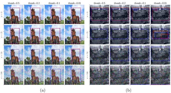
4.6 Priming vs. Pruning. Priming a detector allows it to find ob-jects in images with high levels of noise while mostly avoiding false-alarms. Left to right (a,b): decreasing detection thresh-olds (increasing sensitivity). Top to bottom: increasing levels of noise. Priming (blue dashed boxes) is able to detect the horse (a) across all levels of noise, while pruning (red dashed boxes) does not. For the highest noise level, the original classifier does not detect the horse at all - so pruning is ineffective. (b) Priming enables detection of the train for all but the most severe level of noise. Decreasing the threshold for pruning only produces false alarms. We recommend viewing this figure in color on-line. . . 91 4.7 Effect of priming a segmentation network with different cues. In

each row, we see an input image and the output of the network when given different cues. Top row: cues are respectively bottle, dining table, person. Bottom row: cues are respectively bus, car, person. Given a cue (e.g, bottle), the network becomes more sensitive to bottle-like image structures while suppressing others. This happens not by discarding results but rather by affecting computation starting from the early layers. . . 95

(20)

4.8 Comparing different methods of using a cue to improve seg-mentation: From left to right: input image (with cue overlayed), ground-truth (all classes), unprimed segmentation, pruning type-2, pruning type-1, and priming. In each image, we aid the segmentation network by adding a cue (e.g, “plane”). White regions are marked as “don’t care” in the ground truth. . . . 96 4.9 Priming a network allows discovery of small objects which are

completely missed by the baseline method or ones with uncom-mon appearance (last row). From left to right: input image, ground-truth, baseline segmentation [4], primed network. . . 98 5.1 Illustration of the modular information flow of the Selective

Segmentation Network (SSN) at each processing stage of the inference and learning phases. The stages in orange belong to the inference phase at which given some unknown test image, the predicted segmentation outputs are returned. The stages in yellow represent the learning phase at which SSN parameters are learned. The text provides details for each of the figure panels.107 5.2 Illustration of SSN consisting of multiple parts such as the

feedforward BU representation, the classification LSD module, the TD selection network, and the up-sampling segmentation pipeline. Arrows show the information flow from one part to another part at the learning phase. The input and output at each stage are labeled using the variables which are defined in the subsequent sections. . . 111

(21)

5.3 The BU network defined using the AlexNet and VGG-16 con-volutional neural network architectures on the right and left respectively. The green box over the input image is the total receptive field size of a unit on the top feature map h. Blue boxes are pooling layers and the black boxes are convolutional layers with ReLU activation functions. Since the total receptive field size is smaller than the input image size, the top feature maps have size of greater than 1. . . 112 5.4 Parallel (right) and Sequential (left) architecture approaches to

design the Loose Spatial Detection (LSD) module. Each shade of blue represents a group of layers with the intermediate layers

li, the output prediction layers ci and the output score maps

si. The top feature layer is the last layer of the BU network that outputs the feature maps h. The layer connectivity of the parallel and sequential choices along with the spatial size reduction from one group to another is depicted schematically. 113 5.5 The receptive field size of three LSD groups over the input

fea-ture map h. The shades of blue represent the receptive field and the output score map of a particular group of LSD layer. 114

(22)

5.6 Illustration of the segmentation network with different para-metric and modulation nodes. Each block receives the hidden (blue) and the gating (red) activity inputs. The selective gat-ing units modulate the hidden units at the first node M. At each layer, after input fusion, information is integrated into the main segmentation pipeline using the second modulation node

M. We conduct experiments on three different types of modu-lations: addition, multiplication, and concatenation. The layer label subscripti is neglected for the sake of brevity. . . 125 5.7 Comparison of the segmentation predictions of SSN with FCN

on Pascal dataset. From left to right: RGB images, ground-truth, FCN predictions, SSN predictions. . . 141 5.8 Comparison of the segmentation predictions of SSN with FCN

on CamVid dataset. From left to right: RGB images, ground-truth, FCN predictions, SSN predictions. . . 142 5.9 Comparison of the segmentation predictions of SSN with FCN

on Horse-Cow part parsing dataset. From left to right: RGB images, ground-truth, FCN predictions, SSN predictions. . . . 143 5.10 Demonstrating the role of the number of levels of TD and BU

modulation on the segmentation prediction. From left to right: RGB images, ground-truth, SSN with 1 level of modulation, SSN with 2 levels of modulation, and SSN with 3 levels of mod-ulation respectively. . . 145

(23)

5.11 Robustness of SSN is measured at different interference lev-els (σ) for the uniform (UN), salt-pepper (SP), and box oc-clusion (BO) types. σ determines the bandwidth of the uni-form noise (255 × σ), the probability of having salt-pepper noise at a location, and the length of the occlusion box (σ× min(himage, wimage)) respectively. The modulatory role of the depth of the TD selection is demonstrated for SSN-k with in-puts at k number of levels into the segmentation pipeline. . . 147 5.12 Three different levels of uniform noise is added to the RGB

images. From left to right the noise level is 0.25, 0.45, 0.65 respectively. . . 148 5.13 Three different levels of salt-pepper noise is added to the RGB

images. From left to right the noise level is 0.25, 0.45, 0.65 respectively. . . 148 5.14 Three different levels of box-occlusion noise is added to the RGB

images. From left to right the noise level is 0.25, 0.45, 0.65 respectively. . . 148

(24)

6.1 Schematic illustration of the proposed method for connection pruning that leads to the reduction of the number of network parameters. On the left side, a toy multi-layer feedforward network is shown. On the right, the corresponding TD net-works is given. At each layer, once the active connections ˜ware computed using the TD selection mechanisms, they are addi-tively accumulated into the persistent buffer V; subsequently, the mask tensor M is scheduled to get updated after a number of iterations. The feedforward pass is always additively modu-lated with the mask tensors M. The arrows show the direction of information flow. . . 156 6.2 Detailed demonstration of different stages of computation of

the BU and TD passes for selective connection pruning. At each layer, the inputs to the TD selection unit, the active connections

˜

w, the additive accumulation into the persistent buffer, and the multiplicative mask of the BU kernel weight are depicted. . . . 163 7.1 The TD network modulates the BU feature representation in

the iterative BU pass. The total loss is defined as the weighted sum of the loss of the first and second BU passes. . . 177 7.2 The gating activities at each layer modulate the hidden

(25)

7.3 Illustration of sample digit images in the WMNIST dataset. The red boxes are the predicted bounding boxes using the LeNet-5 BU pass for feature encoding and the TD selection pass for object localization. . . 181 7.4 Demonstration of the effect of the additive uniform noise in the

background and the comparison of the localization performance of the the LeNet-5 reference model (top) with the selective fine-tuned model (bottom). The ground truth and predicted boxes are depicted with the blue and red boxes respectively. The additive noise is taken from a uniform distribution with a lower and upper bounds of 0 and 100 respectively. . . 182 7.5 The effect of the additive noise distortion in the background

on the classification accuracy rate. Ref and SFT refer to the reference and selectively fine-tuned models respectively. The vertical axis represents the robustness of the fine-tuned network at different noise levels. Robustness is calculated by the ratio of the accuracy rates of the noisy images over the clean images. The horizontal axis indicates the maximum amount of pixel intensity the uniform distribution may add to the background pixels. . . 183

(26)

7.6 The effect of the additive noise in the background on the local-ization accuracy rate. Ref and SFT refer to the reference and selective fine-tuned models respectively. The horizontal axis indicates the maximum amount of pixel intensity the uniform distribution may add to the background pixels. Robustness is calculated by the ratio of the accuracy rates of the noisy images over the clean images. . . 184 7.7 Random samples generated by the four noise methods: (a)

Grating: radial grating with random centers, (b) MoG: Mix-ture of Gaussians, (c) Squares: squares with random intensity values, and (d) RLines: short lines with random centers and orientation. . . 186 7.8 Comparing the effect of different methods of generating

con-textual noise perturbation on the classification accuracy. From left to right: (a) Grating: radial grating with random centers, (b) MoG: Mixture of Gaussians, (c) Squares: squares with ran-dom intensity values, and (d) RLines: short lines with ranran-dom centers and orientation. The vertical axis represent the classifi-cation robustness metric, and the horizontal axis represent the maximum pixel intensity the noise adds to the background. . . 187

(27)

7.9 Comparing the effect of different methods of generating con-textual noise perturbation on the localization accuracy. From left to right: (a) Grating: radial grating with random centers, (b) MoG: Mixture of Gaussians, (c) Squares: squares with ran-dom intensity values, and (d) RLines: short lines with ranran-dom centers and orientation. The vertical axis represent the local-ization robustness metric, and the horizontal axis represent the maximum pixel intensity the noise adds to the background. . . 187 7.10 Comparison of the label and bounding box predictions of the

LeNet-5 reference and fine-tuned networks once the background regions is perturbed with four different types of noise meth-ods. In each section, the top and bottom rows represent pre-dictions from the reference and selective fine-tuned networks. The ground truth and predicted bounding boxes are illustrated with blue and red boxes respectively. The ground truth and predicted labels are shown at the top-left and top-right of their corresponding box respectively. . . 188

(28)

7.11 Comparison of the label and bounding box predictions of the AlexNet reference and fine-tuned networks once the background regions is perturbed with four different types of noise meth-ods. In each section, the top and bottom rows represent pre-dictions from the reference and selective fine-tuned networks. The ground truth and predicted bounding boxes are illustrated with blue and red boxes respectively. The ground truth and predicted labels are shown at the top-left and top-right of their corresponding box respectively. . . 189 A.1 Illustration of STNet localization performance for both

VG-GNet and GoogleNet. The top, middle, and bottom row of each section contains images demonstrating the ground truth bounding boxes, bounding box predictions of ST-VGGNet, and ST-GoogleNet respectively. . . 234 A.2 Unsuccessful localization cases based on STNet bounding box

predictions are demonstrated. Multi-Instance and Correlated Accompanying Object scenarios are the two main sources of STNet unsuccessful localization. Each section contains image rows for ground truth, ST-VGGNet and ST-GoogleNet bound-ing boxes from top to bottom. . . 235 A.3 Class Hypothesis Visualization using STNet. In each section,

the top row contains RGB images depicting ground truth bound-ing boxes, and the middle and bottom row contains the CH maps from ST-VGGNet and ST-GoogleNet respectively. . . . 236

(29)

A.4 The effect of the context inference imposed by the learned repre-sentation is illustrated in the CH maps given in the bottom rows of each section. The middle row contains the CH maps from the original proposal of ST-VGGNet. The top row provides RGB images with the color-coded bounding boxes. Blue boxes are taken from the ground truth. Green and red boxes represent original and partially-deactivated ST-VGGNet predictions. . . 237 A.5 Correlated accompanying objects prioritize localization of

re-gions outside the ground truth according to the learned repre-sentation. In each section, the top row contains RGB images with the ground truth boxes (blue). The red boxes are proposed by the modified ST-VGGNet. . . 238 A.6 The location of the cat from Fig. 4.1 in Chapter 4 . . . 239 A.7 Additional effects of priming with the SSD [5] object detection

network. Each 4x4 block of images shows the detections of the unprimed-network in red and of the primed network in blue. From left to right, the detection threshold is decreased, allowing less confident score to appear, while also surfacing false alarms. From top to bottom, the level of noise increases. A primed network detects objects in noisy image more robustly than an unprimed one. . . 241

(30)

A.8 Additional effects of Priming with the deeplab[4] segmentation network. Each four columns shows from left to right: input im-age, ground truth segmentation of a specific class, result of un-primed network, result of un-primed network using proposed method.242

(31)

Chapter 1 Introduction

Vision has long been recognized as one of the major input modalities for the hu-man brain with striking physiological and psychophysical capabilities enabling sensation, perception, cognition, and action. Vision consumes a large portion of the human brain processing resources in comparison with other modalities such as audition and olfaction. This underscores the critical role that vision plays in the definition of an intelligent system. The human brain receives a high volume of visual sensory data, and as a result, has developed special-ized and complicated information processing machinery to support complex decision situations.

The scientific community has conducted a large amount of inter-disciplinary research in different academic fields such as neuroscience, cognitive science, and computer science to not only find answers to questions but also discover unknown aspects of the brain information processing system. Among various cognitive capabilities such as learning, memory, reasoning, and planning,

(32)

at-tention plays a critical role. Atat-tention enables us to selectively concentrate on an aspect of the input stream while ignoring others. Due to the large amount of sensory data received at any moment by the human brain, attention is effec-tively engaged as a crucial component in the efficiency and speed of the entire processing pipeline [6, 7, 8].

The ability to formulate spatial relationships and functional interactions of object categories is an integral component of any intelligent machine. Different generic recognition tasks such as object classification, localization, detection, and segmentation are collectively important to accomplish short- and long-range task objectives for an intelligent vision system. The recent success of machine vision systems is impactd by the improvement in the performance of such recognition tasks [9, 10].

The current dominant approaches to model visual recognition tasks are mainly inspired from the feed-forward pass of information processing in the visual cortex. Information flows from the early stages of sensory data recep-tion to an intermediate representarecep-tion and finally the top semantic-encoding levels. While the feed-forward pass plays a central role in forming a visual representation, this has been shown in various experimental studies to be in-complete. It is accepted that not only does information flow forward from the bottom to the top of the visual hierarchy, but also top-down connections prop-agating information in the reverse direction are widely established throughout the visual hierarchy. [11, 12, 13, 14]

In human and machine vision systems, two directions of information pro-cessing flows are commonly recognized: a data-driven or feed-forward

(33)

direc-tion (Bottom-Up), and a reverse direcdirec-tion (Top-Down) that has a predictive, controlling or modulatory role. The sensory input data is processed in the Bottom-Up (BU) pathway and sequentially transformed into high-level se-mantic information such that some task criterion is satisfied. The Top-Down (TD) direction provides a route for knowledge, goals, priorities and context to be included in relevant processing stages throughout the visual system. We use feed-forward, bottom-up, and data-driven interchangeably in this docu-ment to refer to the parametric multi-layer transformation of the input data to the output semantic information. In the following, we introduce the con-tributions of the thesis in sequential order. Chapter 2 will provide the basics of the neural network machinery and then overview the related approaches to visual attention modeling in neural networks for visual recognition tasks.

Chapter 3 - Top-Down Selection: Visual attention is one of the sources that activates the modulatory top-down processing. The goal is that depend-ing on task requirements, some level of the visual hierarchy needs to be mod-ulated or tuned according to the high-level semantic information computed at the top of the hierarchy. The propagation, formulation, and operation that jointly develop the systematic modulation form the essence of Top-Down vi-sual attention. The major goal of the thesis is to investigate, explore, and formulate in a systematic approach a top-down selection mechanism for con-volutional neural networks to facilitate attentional modulations. The critical element of an attentional modulation mechanism is the computation of the se-lection patterns based on which network responses at multiple layers are tuned. Top-Down selection is among the set of mechanisms that jointly define the

(34)

vi-sual attention framework proposed by [7]. The role of selection mechanisms is to determine the most important sub-set of the network processing units and parameters according to some task criteria. We present a novel Top-Down attention framework with hierarchical selection mechanisms for convolutional neural networks in Chapter 3 and perform experimental evaluation on the task of object localization.

Chapter 4 - Priming Neural Networks: Visual task priming is an early tuning process before the feedforward information flow in the visual hierarchy. The objective is to tune the visual hierarchy to be prepared for the expected stimulus and thus enable the visual hierarchy to optimally process it. One purpose of visual priming is to help detection of unnoticeable scene elements under severe and misleading visual conditions such as contextual noise and camouflaged objects. We propose a top-down mechanism in the convolutional neural network framework to mimic the process of priming in the context of object detection and segmentation in Chapter 4. This implicit top-down mechanism shapes the bases of the subsequent chapters in which we introduce the explicit top-down selection mechanisms for related visual tasks.

Chapter 5 - Object Segmentation Using Selective Attention: De-spite recent success of purely feed-forward models, several aspects of perfor-mance degradation in Bottom-Up (BU) networks have been uncovered. Re-search on visual confusion and adversarial attacks [15, 16, 17, 18, 19] have revealed the vulnerability of data-driven feedforward networks. Furthermore, signal interference issues within multi-layer hierarchical representations are well studied and reported in the literature [20, 21, 22]. Some of these

(35)

con-volutional neural network problems might be due to signal interference issues within such data-driven hierarchical representation. Additionally, these mod-els are sensitive to small input perturbations and are easily fooled for arbitrary final label predictions. In Chapter 5, we propose to extend the TD selection mechanism for the task of semantic segmentation. We test the hypothesis that a convolutional neural network augmented with a TD modulatory and controlling mechanism can achieve better data generalization and be more ro-bust against out-of-distribution perturbations for object segmentation. The attention-driven feature modulation is built on top of the proposed TD se-lection mechanisms for object segmentation. We experimentally validate the observation that the modulation of the BU features initiated by TD selection improve the benchmark performance metrics in comparison with the baseline model on benchmark dataset.

Chapter 6 - Attention for Compact Neural Representation: The widespread usage of mobile platforms with improved video-recording capabil-ities have demanded applications with intelligent visual features to be able to process large amounts of data instantly. Neural network compression based on some form of sparsity over the parameter space may provide a route to this goal. The idea is to prune redundant network connections and consequently leave the influential connections intact to maintain network inference accu-racy while reducing the redundancy for the sake of a minor compromise of performance loss. Our proposed attentional framework in neural networks is extended to investigate the hypothesis whether such top-down mechanisms are informative to drive the pruning of neural networks. We develop an

(36)

attention-driven connection pruning approach for the convolutional neural net-work framenet-work in Chapter 6 and show the parameter reduction is competitive with the baseline approaches.

Chapter 7 - Contextual Interference Reduction: Contextual inter-ference with the foreground target objects is one of the main shortcomings of current neural networks. Due to the dense hierarchical parametrization of convolutional neural networks, “cross talk” of the foreground and the back-ground representation is inevitable [21]. The category label prediction using convolutional networks relies on feature extraction performed uniformly across the input image. Consequently, there is no explicit notion of contextual in-terference reduction in such models. In Chapter 7, we propose a systematic approach to shift learned neural representations towards the foreground target objects in order to achieve a higher degree of representation dis-entanglement for object classification. We define a selective fine-tuning of neural networks using a unified bottom-up and top-down framework. A gating mechanism of hidden activities is defined in the iterative feedforward pass. An attention-augmented loss function is introduced that permits the network parameters to be fine-tuned for a number of iterations. The fine-tuning using the itera-tive pass helps the network to reduce the contextual representation emphasis. Therefore, the label prediction relies more on the target object representation and consequently achieves a higher degree of robustness to the background changes. The experimental evaluations on a modified MNIST dataset reveal not only that the results are improved but also a higher degree of robustness to background additive noise is obtained.

(37)

To conclude, the significance of the research is two fold: First, we present a unified network with both BU and TD information processing pathways. A novel TD selection mechanism using multiple computational stages is intro-duced. Second, we conduct research to gain more reliable insights towards the computational role of a TD pass in the conjunction with a BU pass for differ-ent visual tasks such as object localization, detection, and segmdiffer-entation. The significant role of the proposed TD selection mechanism is demonstrated for different tasks with respect to baseline models and compared under different input distortion scenarios.

(38)

Chapter 2 Background

In this chapter, we review the literature related to the thesis. We first define the terminology used in the thesis in Sec. 2.1. We then introduce the bases and foundations of the neural network framework for different visual recognition tasks such as object classification, detection, and localization in Sec. 2.2. We define the terminologies, computational elements, and modeling approaches to develop neural network models for such tasks. In Sec. 2.3, previous visual attention modeling attempts and approaches will be reviewed.

2.1 Introduction

Object recognition tasks have been heavily studied in various research disci-plines ranging from psychology, cognitive science, and neuroscience, to com-puter science. In comcom-puter science, the primary goal is to develop a compu-tational machinery based on a solid understanding of different visual tasks. The secondary goal has been to develop machine vision systems that

(39)

com-pete with human performance; this has proven to be very challenging. In our definition, we refer to object recognition as a general task that involves two different types of tasks; object instance recognition and object class recogni-tion. The first type is a matching problem such that previously seen object instances have to be identified under some variable imaging conditions and partial occlusions based on a bank of visited exemplars. Image alignment and registration processes also are often required. For example, recognizing the face of a particular person under different conditions is defined as object instance recognition.

The second type, also known as category-level or generic object recogni-tion, aims to recognize instances of learned categories. The apparent difference is that in the latter, the target instances are unseen by the recognition model and the generalization capability is important. However, in the former, a par-ticular instance is known and the goal is to identify it under various conditions. Following Perona’s [23] definitions, we refer to the object instance recognition as the Verification task and the object class recognition as either Detection or Classification. Both detection and classification can be augmented with the object localization task. Object localization is defined as the task of spatially localizing a target object in the input image [23]. In other words, the answer to the question of “where is a target object?” satisfies the localization task requirement.

Perona [23] defines object classification as: given an image patch, what object category label, from a set of predefined categories, best represents the patch content? The objective is very straightforward in the sense that the

(40)

output is produced as the predicted label of the given image patch. The assumption of this task obviously is that the patch should reflect the object and the context it resides in. Depending on how much context surrounds objects in input images, localization could be non-trivial.

Object recognition tasks performed by the human visual system in a real-life scenario is even more challenging. An object in a real-world scene is often perceived by a human observer in a cluttered environment with lighting and shading variations. The detection of an instance of some object category in a noisy cluttered environment with partial occlusion makes the task of object detection more complicated. A detection model predicts whether instances of some particular object category exist in the input images. Following the requirements defined for the detection tasks [24, 25], object detection always requires the localization of the detected instances. However, localization for object classification is explicitly mentioned if required. The single-object lo-calization task is one of the challenges defined for the ImageNet benchmark dataset [24] and it explicitly requires location prediction on top of object clas-sification.

Visual variations are transformations in the spatial domain that make recognition very challenging. All types of visual variations can be divided into two distinct groups: object variations and image variations. Object vari-ations work within a category delimiting different instances based on visual cues such as color, texture, shape, pose, and size. However, image variations are caused by different lighting, place, atmospheric (weather), illumination, and viewpoint conditions. Object variations can change one instance of a

(41)

category to another instance while image variations always keep the instance identity intact. The variation by the viewpoint condition is separate from the object pose variation. It is due to the fact that viewpoint variation is caused by the external observer while the object pose variation is produced by the structural variation of the object itself. Therefore the former is purely independent from the nature of object categories while the latter is inherent in object categories. Nonetheless, recovering the pose of an object is usually preceded by an estimation of the viewpoint parameters.

Object categories can further be distinguished according to their structural configurations. Horse, dog, chair, book categories are instances of deformable or structured object categories. On the other hand, amorphous or unstruc-tured categories do not have constant shape or size such as cloud, sky, grass categories. Consequently, they can be described in terms of local appearances based on color and textural patterns. They are called things and stuff semantic categories respectively in [26].

The first and most critical step towards solving object recognition prob-lems generally is the choice of visual representation for input images. Moving from low-level raw representation of gray-scale, color, gradient, local shape and texture cues to a mid-level feature representation is a very challenging task. Objects could be represented in the 2D image domain based on explicit shape and form cues, which rely on the boundary depiction of the objects dis-tinguishing them from the background, or based on the visual appearance of the object surface. Following each would lead to either shape-based models or appearance-based models respectively.

(42)

2.2 Object Recognition with Convolutional

Net-works

By defining object classification as the task of predicting the category label of an input image, the crucial part is to learn a visual representation suitable for invariant object classification. Variability in this task ranges from object to image variations. Robustness to such variations is the key aspect of a reliable representation. Dealing with object location variation within the image frame is very important. It could be, however, overcome by framing the object of interest in the center of the input image or by injecting very slight shift invari-ance into the representation model so then the object location shift would be tolerated within the image frame. A visual hierarchy is defined as a system-atic organization of multiple levels of feature extraction, grouping, selection, and integration into a unified framework. The objective of the hierarchy is to be able to represent input data according to some task requirements and specifications.

In the neural network modeling paradigm, object classification method-ologies consist of two main components: the visual representation and the discriminative classifier. Visual representations are categorized based on the depth of visual representations ranging from shallow to deep representations. The intuition is that the depth of the visual representation would help to bet-ter encode the semantic and appearance factors. Various attempts to visual representation modeling for object recognition can be differentiated by the con-sideration of the architecture criteria such as the depth of the representation

(43)

defined by the number of filtering, sub-sampling, pooling, and non-linearity layers. The type of operation at each layer in addition to the intrinsic pa-rameter settings is another aspect of representation modeling. Whether the hierarchy parameters are defined to be hard-wired or learned in a supervised or unsupervised manner matters when characterizing one approach from an-other. Lastly, the modeling framework that imposes the objective criterion onto the underlying representation plays an important role. The classification paradigm characterizes the objective terms, the optimization routines, and the parameter updating procedures.

A visual representation is defined as a transformation function φ(I) that encodes the input image I to some form of vectorial representation in a high-dimensional space. A robust nonlinear representation is capable of projecting the input space to a feature space such that visual tasks can be performed using a linear decision machine. Manifold learning of a visual representation hypothesizes that a robust visual representation transforms a tangled high-dimensional input space into a feature space such that the input data samples lie on linearly separable manifolds.

Convolutional Neural Networks have been studied from different perspec-tives ranging from a biological point of view in neuroscience to a computational point of view in computer science. In analogy to the brain, the basic opera-tion of weight sharing implemented in convoluopera-tional neural networks can be regarded as the representation of a particular salient feature over the reti-nal topography in one visual cortical area. The basic selectivity of neurons achieved through their receptive field profile can be regarded as the

(44)

convolu-tion operaconvolu-tion in such networks. [27] is one of the first attempts to propose a computational model with convolutional connectivities. It was, however, formulated to suit unsupervised learning problems. A more extensive realiza-tion of convolurealiza-tional networks in the computer vision applicarealiza-tion of isolated character recognition was appeared in [28, 29] purposefully oriented for su-pervised learning problems. The network architecture named LeNet-5 shows how a well-implemented convolutional visual hierarchy with the representation learned through a particular optimization procedure can be successful in a real computer vision application.

The breakthrough of convolutional networks in large-scale object recogni-tion competirecogni-tions started with the inspirarecogni-tional work of [30], which is com-monly referred to as AlexNet. The trained convolutional network was one of the largest and well-implemented networks to date with the best performance results on popular benchmark datasets. The highly GPU-optimized implemen-tation of convolutional networks has been very highly effective. The overall computation throughout the hierarchy of convolutional networks is such that local parallel units can be utilized to achieve a major processing speedup in both the learning and inference stages. GPUs are designed to have many local parallel processing units that can be assigned to perform the computa-tion required for multiple nodes simultaneously in a convolucomputa-tional network. The use of Rectified Linear Units (ReLU) [31] as a novel non-linearity and a regularization method called Dropout [32] to reduce over-fitting in the fully-connected layers are among the important breakthroughs in the advances of neural networks.

(45)

2.2.1 The Basic Building Blocks

Convolutional networks are comprised of a modular combination of different types of layers on top of each other beginning from an input layer and ending with a score function based on which the loss function is measured according to the label of the input data.

Convolutional networks are comprised of various stages of processing con-secutively processed in a cascade manner on top of each other forming the visual hierarchy. The convolution operation through a particular kernel profile is the essence of feature selectivity. A non-linear activation function is applied in the next stage to compute the output of model neurons (hidden units) at each layer. This is usually followed by another type of layer called pooling and sub-sampling layers to impose some level of gradual shift invariance.

Convolutional Layers: The first type of layer is the convolutional layer, the core building block of convolutional networks. By analogy to the receptive field selectivity of the neurons in visual cortex, the basic operation of weight sharing implemented in convolutional networks leads to the representation of a particular type of feature over the retina topography in a visual cortex area. In other words, the basic selectivity of neurons through their receptive field profile can be regarded as the convolution operation in such networks. The convolution operation is the means through which the feature selectivity is locally applied. Convolutional layers are characterized by design choices such as kernel size, number of input feature channels, number of output feature channels, stride, and border padding. Fully-connected (FC) layers are 1×1

(46)

layers inspired by MLP networks. Hidden nodes in FC layers are connected to all of the hidden units in the previous layer. A matrix multiplication added with a bias offset is needed to compute activities in a FC layer. The output feature channels of the last FC layer is equal to the number of categories in classification problems. It learns to encode for the class scores, which are arbitrary real-valued numbers. There is no activation function after the last FC layer but rather the logistic regression (for binary classification problems) or softmax layer (for multi-label classification problems) to generate predictive probability values.

Non-linearity Layers: The other layer type, mostly used after the con-volution layer, is the non-linear activation function. The idea is based on the biological inspiration of real neurons for which the firing rate of neurons is lim-ited between zero and a positive clamping value [33]. Once the output maps are computed by a convolutional layer, a transfer function is applied to map the input to a proper neural response range. Sigmoid andT anhare the most common functions used in the early days. Rectified Linear Units (ReLU) [31] is simply a linear function such that the values lower than a threshold are set to zero. To overcome the shortcomings of ReLU such as the zero gradients for value lower than zero, different ReLU variants have been proposed such as the Parametric ReLU (PReLU) [34], the Leaky ReLU (LReLU) [35].

Hidden Normalization Layers: One modeling inspiration from the real neuronal mechanisms observed in neuroscience research is inhibition processes such as lateral inhibition. There are different attempts to address the need for a similar mechanism in convolutional neural networks. Local Response

(47)

Normalization (LRN) [30] and Local Contrast Normalization (LCN) [36] are among the first attempts to investigate the role of normalization layer in neu-ral networks. They implement a similar idea with a subtle difference in terms of the scope of normalization and also whether it is just divisive or also sub-tractive too. Such normalization is applied after non-linearity layers in certain layers to stabilize training and improve generalization. Unlike these two meth-ods with small normalization scopes, Batch Normalization (BN) layer [37] is proposed with a more global scope of normalization to mainly deal with im-proper parameter initialization and lack of training consistency, and it usu-ally comes after ReLU layers. Since the batch concept is not always present, Layer [38], Instance [39], and Group [40] normalization layers are proposed to avoid exploiting directly the batch dimension. The overall core idea is to collect statistics across the input hidden tensors according to some grouping approach (e.g. batch dimension in BN), and then use them to normalize the input hidden tensors in a divisive and subtractive manner followed by some parametric scaling and addition. [41] recently proposes a synchronized BN layer that collects statistics and updates coefficient parameters across multi-ple GPUs when the mini-batch size is high (e.g. 128) and each GPU holds one input sample due to a large network or input data size.

Pooling Layers: Pooling layers are utilized as an attempt to inject small local shift invariance into the overall representation by the gradual pooling mechanism. Average and Max pooling [42] are the two popular widely used pooling layers, which spatially pool information across a 2D window of hidden units on a feature map. Properties such as kernel size and sub-sampling stride

(48)

are important. In contrast to the spatial pooling approaches, Maxout [43] is regarded as a pooling operation over the inter-channel dimension. Other vari-ants such as Probabilistic Maxout (Probout) [44], Probabilistic Max-Pooling [45], p-norm pooling [46], and parametric p-norm pooling [47] are proposed in the hope of improving their invariance properties. Network in Network (NIN) [48] is proposed to incorporate a higher degree of complexity in the pro-file selectivity of hidden units in convolutional networks. It replaces a simple weighted summation performed by convolution with a Multi Layer Perceptron (MLP) motivated layer to add more complexity for feature encoding. NIN is respected as a cross-channel parametric pooling and is extended by [49] into a new architecture using Inception modules. The idea is to use a set of 1×1 convolution filter banks to reduce the number of input feature maps into a lower more computationally affordable number for the subsequent k ×k fil-ter banks. A particular incarnation of the inception modular architecture is called GoogLeNet and introduced in [49]. Residual networks [50] are proposed as a way of overcoming the obstacle of losing gradient information in convo-lutional networks using skip connections. Inspired by the Spatial Pyramid Kernel Matching [51], Spatial Pyramid Pooling (SPP) [52] is defined to over-come the variable image size issue by a pooling layer that outputs fixed-length feature maps.

Training and Testing Protocol: A popular learning algorithm for con-volutional neural networks is to minimize a loss function over the training set. This is a non-linear optimization problem that is done using iterative gradi-ent descgradi-ent optimization updates. The goal is to update parameters with the

(49)

gradients that minimize the loss function. Basically a best direction based on which a particular parameter should be changed is the one given by the first partial derivative of the loss function with respect to the parameter. The chain rule is a systematic approach to analytically compute error gradients of network parameters. It is interchangeably referred to as Backpropagation in the neural network community [53]. Having the input data propagated into the feed-forward layer throughout the network at the inference phase, error gradients of the weight parameters are analytically computed according to an objective function and systematically propagated backward from one layer to the next. Once gradients are computed, the gradient optimization algorithm updates the weight parameters and repeats these steps for the next set of training samples.

Network Regularization: As the capacity of a network in terms of free parameters increases, the model tries to memorize the training data set rather than to learn the underlying data distribution. This is famously known as over-fitting and will lead to low generalization performance at the testing phase. In order to avoid over-fitting, various regularization methods have been proposed such as the weight-decay approach (L1- or L2-norm). It is imposed on the objective loss function at the learning phase to regularize weight parameters. Early stopping is also one of the early proposals. Dropout [32, 54] is proposed to decrease the co-adaption that emerges during the training phase between hidden units by randomly setting hidden units to zero. Adaptive Dropout [55] uses an auxiliary network to learn the probability based on which dropout mask is generated for each hidden uni. DropConnect [56] set the connection

(50)

weights rather than the hidden units to zero .

Network Representation Visualization: Understanding the hierarchi-cal representation of convolutional neural networks plays a critihierarchi-cal role. [57, 58] propose to define pooling switches recorded in the feedforward pass and are used to project back to the top layer activities to the input layer using the De-convolution layers. [59] proposes a gradient-based visualization method that uses automatic differentiation of the loss function with respect to the input layer. The idea of activation maximization simply is to maximize the classifi-cation score of a specific class label penalized with some regularization term such as L2-norm term for the input image. The regularization terms act as image priors that restrict the search process in the input image space to those that can resemble well natural images. In addition to the hand-designed nat-ural image priors [60, 61, 62]such as Gaussian blur and α-norm, [63] proposes a learned prior based on Generative Adversarial Networks (GAN) [64]. This learned prior provides high-quality input image search results and intermediate hidden activity visualizations.

2.3 Visual Attention in Deep Learning for

Ob-ject Recognition

Attention in humans helps to concentrate and tune the brain’s computational resources to fulfill task requirements within a particular time frame. Object detection in a large context is a task that inherently demands a form of pro-cessing concentration. In a real life scenario, object detection is regarded as

(51)

finding instances of a particular category in a noisy, cluttered, and complex visual environment. The task of finding a car on the street among many dif-ferent irrelevant object categories and then consequently be able to localize it, is an example of the goal approached in object detection with localization. One question that emerges at this point is whether the localization is by itself a task separate from the detection task. Is it that first an object is detected out of noisy context and then, upon the requirement of the task, is localized? Or is it that detection is performed on a localized portion of input image, and thus, localization is achieved a priori to detection? These two extreme points form the two sides of the spectrum of approaches for object detection. We call them late- and early-localization approaches respectively.

2.3.1 Early-Localization: Hypothesizing for Objectness

Early-localization measures some generic definition of objectness from local and pictorial cues in an image, and then outputs an importance map of the regions that are most likely to contain category objects. Objectness indicates how likely a category object exists across image regions [65, 66]. A subtle ques-tion is what is the best metric to measure objectness, and what differentiates object categories for which ground-truth labels are provided from the unla-beled ones. A detection system utilizes the objectness measurement to pick the most salient regions to attend to for category prediction. Refinement over background regions and pre-trained visual representation seems necessary to help early-localization approaches beat the state-of-the-art in object detection. It is worth mentioning that the weak early-localization approach is equivalent

(52)

to the brute-force sliding window approach to output importance maps over which candidate regions containing objects are returned. On the other hand, a strong early-localization approach achieves the 100% recall accuracy with a number of bounding box proposals equivalent to the number of ground truth bounding boxes. In other words, the highest level of recall accuracy is achieved with the least number of proposals using the strong approach.

A measure of objectness is provided over the entire high resolution image using a class-agnostic algorithm in order to model a level of attention for the classifier that predicts category labels. Objectness models work in the bottom-up fashion without utilizing any form of top-down task knowledge. They rather collect and integrate pictorial and structural information locally from different tracks of visual processing to find regions with a high measurement of objectness.

Approaches for object proposal generation can be categorized into three distinct paradigms. The first one is harnessing the image pictorial structure locally and globally to merge the super-pixels into a hierarchy [67, 68, 69, 70]. Cutting through the hierarchy at some specific level provides a number of bounding box proposals. We will explain this approach in more detail in Sec. 2.3.1.2. The second paradigm is measuring objectness of boxes through a learn-ing method. It is intrinsically statistically data-driven [66, 71, 72, 73]. Uslearn-ing a pre-trained visual representation, objectness is learned in a class-generic man-ner. This is similar to the simultaneous detection and segmentation method-ology. Further information is given in Sec. 2.3.1.3. Lastly, based on the classic figure/ground criteria, the third paradigm uses segmentation algorithms which

(53)

are used to partition input images spatially into distinct regions [74, 75, 76]. The bounding boxes enclosing the partitions are proposed for object classifi-cation. This approach is expanded in more detail in Sec. 2.3.1.3.

2.3.1.1 Metrics to Measure Objectness

Objectness detection algorithms are interchangeably referred to as bounding-box proposal algorithms. The intuition is to use an objectness measure and other factors to confidently propose regions in boxes that most likely span the entire extent of the objects in an image. Three evaluation measurements are commonly characterized in the performance comparison of different al-gorithms. First, the recall rate is defined as the accuracy of hitting correct ground-truth bounding boxes from the set of proposals regardless of the false positive rate. There is always a trade-off between false negative and false pos-itive rates. Accounting for one would impact the other. Therefore a good cutting-point threshold is always cross-validated. However, region proposal algorithms are mostly evaluated based on the recall rate. Precision is left over to object classification algorithms. The main criterion is to increase the recall as much as possible.

The second evaluation metric is the number of proposals to achieve a par-ticular level of recall. A powerful reliable objectness detector is recognized based on the number of proposal boxes. Apparently, as the number increases, the object classification module takes more time and gradually shifts towards the brute-force sliding window search mode. Hence, a decent close-to-optimal objectness detector is the one that while maintaining a low number of

(54)

propos-als, hits the highest recall rate of one.

Third, the size accuracy of the proposals measures objectness detection performance. Tightness of the proposals could be relative and gets refined in the recognition step according to the relative shift invariability of robust classifiers. In practice, recall rate is measured as the total number of proposed bounding boxes that have overlaps of more than some threshold (mostly 0.5) with the ground truth bounding boxes.

2.3.1.2 Harnessing the Pictorial Cues in a Hierarchy

Selective Search (SS) [67] is inspired by the segmentation community to use lo-cal cues to separate figures from ground. SS combines the best of segmentation with a selective search over various locations in the image. Complementary grouping criteria and invariant color spaces are used to diversify the search over the entire space for targeting better regions. SS attempts to use segmen-tation to narrow down the large search space over locations, aspect ratios, and sizes. Rather than the common goal of proposing a strong segmentation strat-egy to partition regions apart, SS uses various strategies to extract knowledge from various aspects of an image ranging from shape, color, curvature, texture. In this regard, there is huge similarity in the representation space of SS with saliency prediction algorithms. These image clues are grouped systematically in a bottom-up manner to generate good object locations using a diverse set of strategies. A fast graph-based algorithm [68] is used to initialize SS. Then a greedy grouping algorithm is iteratively used to construct the hierarchy of regions until the entire image is grouped into one region. Grouping is based on

(55)

the feature similarities of all the neighboring regions and merging of the two most similar ones. This leads to a tree of regions with leaves as the initialized regions and the root as the region covering the entire image. The similarity based on a variety of complementary measures are constrained to be fast such that the measures can be propagated through the hierarchy so then at each level the similarity can be computed from the measures of the previous level rather than the measure from image pixels.

One of the diversification strategies in SS is the utilization of various color spaces with different invariance properties. The second strategy is to use four similarity measures between regions: color, texture, region size, cross-region similarity for combination. The combination of these four measures of similar-ity is used to diversify the search. The third strategy is to generate different starting regions via varying the threshold of the graph-based over-segmentation algorithm. Different ordered sets of proposals are generated according to the diversification strategies. Then regions are extracted for proposal based on their overall ranking.

A multi-scale hierarchical segmentation and object hypothesis generation system in a unified framework called Multi-scale Combinatorial Grouping (MCG) is proposed in [69]. First, a fast normalized cuts algorithm is pro-posed. A set of local contour cues are extracted as the input to the algorithm. Then, a high-performance hierarchical segmentation approach that leverages effective use of multi-scale information is employed. Finally, exploring the combinatorial space of possible object candidates, regions are combined effi-ciently to account for the accurate proposals. Two steps are taken to reduce

(56)

the number of candidates while keeping the quality. One is through combina-torial grouping problem formulation and the other through training a random forest regressor from the low-level bottom-up features to predict the overlap of the region with the ground truth.

MCG differs from SS in focusing on multi-scale information rather than color spaces to generate various hierarchies to diversify the object search. Moreover, pixel accuracy region extraction is more considered in MCG in con-trast to SS. MCG outputs regions whereas SS outputs directly bounding-boxes. However, a normalized evaluation measure which consists of the overlapping area, the number of proposals, and the execution time has to be employed for a fair comparison of different algorithms. Object hypothesis proposals are not meant for accurate categorization result but speed and smaller accurate number of candidates for an optimal object recognition system. It is stated that MCG is marginally better than SS in terms of the amount of the overlap of the proposals with the ground truth.

The Edge Box algorithm is proposed to generate bounding boxes contain-ing objects uscontain-ing edges [70]. Edges are directly used rather than segmented regions, as an informative representation in a non-hierarchical fashion to mea-sure if an object is enclosed in a box. The efficiency of computing edge maps and the sparse representation have made them a promising approach. The number of completely enclosed contours indicates the likelihood of an object in a box. Contour straddling is considered as the sign of a partially enclos-ing object. Thus such contours are removed durenclos-ing the process of scorenclos-ing the completeendres2010categoryly enclosed contours. The issue of how to search