University of Windsor University of Windsor
Scholarship at UWindsor
Scholarship at UWindsor
Electronic Theses and Dissertations Theses, Dissertations, and Major Papers
2010
Microarray time-series data clustering via gene expression profile
Microarray time-series data clustering via gene expression profile
alignment
alignment
K M Numanul Hoque Subhani University of Windsor
Follow this and additional works at: https://scholar.uwindsor.ca/etd
Recommended Citation Recommended Citation
Subhani, K M Numanul Hoque, "Microarray time-series data clustering via gene expression profile alignment" (2010). Electronic Theses and Dissertations. 8060.
https://scholar.uwindsor.ca/etd/8060
This online database contains the full-text of PhD dissertations and Masters’ theses of University of Windsor students from 1954 forward. These documents are made available for personal study and research purposes only, in accordance with the Canadian Copyright Act and the Creative Commons license—CC BY-NC-ND (Attribution, Non-Commercial, No Derivative Works). Under this license, works must always be attributed to the copyright holder (original author), cannot be used for any commercial purposes, and may not be altered. Any other use would require the permission of the copyright holder. Students may inquire about withdrawing their dissertation and/or thesis from this database. For additional inquiries, please contact the repository administrator via email
Microarray Time-Series Data
Clustering via Gene Expression
Profile Alignment
by
K M Numanul Hoque Subhani
A Thesis
Submitted to the Faculty of Graduate Studies
through Computer Science
in partial fulfilment of the requirements for
the Degree of Master of Science at the
University of Windsor
Windsor, Ontario, Canada
2010
1 * 1
Library and Archives Biblioth&que et Canada Archives Canada
Published Heritage Direction du
Branch Patrimoine de l'6dition 395 Wellington Street 395, rue Wellington Ottawa ON K1A 0N4 Ottawa ON K1A 0N4
Canada Canada
Your file Votre reference ISBN: 978-0-494-62711-2 Our Trie Notre r6f6mnce ISBN: 978-0-494-62711-2
NOTICE:
The author has granted a
non-exclusive license allowing Library and Archives Canada to reproduce, publish, archive, preserve, conserve, communicate to the public by
telecommunication or on the Internet, loan, distribute and sell theses
worldwide, for commercial or non-commercial purposes, in microform, paper, electronic and/or any other formats.
AVIS:
L'auteur a accorde une licence non exclusive permettant a la Bibliotheque et Archives Canada de reproduire, publier, archiver, sauvegarder, conserver, transmettre au public par telecommunication ou par I'lnternet, preter, distribuer et vendre des theses partout dans le monde, a des fins commerciales ou autres, sur support microforme, papier, electronique et/ou autres formats.
The author retains copyright ownership and moral rights in this thesis. Neither the thesis nor substantial extracts from it may be printed or otherwise reproduced without the author's permission.
L'auteur conserve la propriete du droit d'auteur et des droits moraux qui protege cette these. Ni la these ni des extraits substantiels de celle-ci ne doivent etre imprimes ou autrement
reproduits sans son autorisation.
In compliance with the Canadian Privacy Act some supporting forms may have been removed from this thesis.
While these forms may be included in the document page count, their removal does not represent any loss of content from the thesis.
Conformement a la loi canadienne sur la protection de la vie privee, quelques formulaires secondaires ont ete enleves de cette these.
Bien que ces formulaires aient inclus dans la pagination, il n'y aura aucun contenu manquant.
Declaration of Co-Authorship
I hereby declare that this thesis incorporates material that is result of joint research, as follows:
This thesis also incorporates the outcome of a joint research undertaken in col-laboration with professors Dr. Alioune Ngom and Dr Conrad Burden (Australian National University) under the supervision of professor Dr Luis Rueda. The collab-oration is covered in Chapter 3 of the thesis. In all cases, the key ideas, primary contributions, experimental designs, data analysis and interpretation, were per-formed by the author, and the contribution of co-authors was primarily through the provision of guidance corrections and constructive criticism.
I am aware of the University of Windsor Senate Policy on Authorship and I certify that I have properly acknowledged the contribution of other researchers t o my thesis, and have obtained written permission from each of the co-author(s) to include the above material(s) in my thesis.
I certify that, with the above qualification, this thesis, and the research t o which it refers, is the product of my own work.
Declaration of Previous Publications
This thesis includes two original papers that have been previously published/submitted for publication in peer reviewed journals (see next page - Table I):
I certify that I have obtained a written permission from the copyright owner(s) to include the above published material(s) in my thesis. I certify that the above material describes work completed during my registration as graduate student at the University of Windsor.
I declare that, t o the best of my knowledge, my thesis does not infringe upon anyone's copyright nor violate any proprietary rights and that any ideas, tech-niques, quotations, or any other material from the work of other people included in my thesis, published or otherwise, are fully acknowledged in accordance with the
Table 1: Declaration of Previous Publications
Thesis Chapter Publication title/full citation Publication status
Chapters 3, 4 N. Subhani, A. Ngom, L. Rueda, C. Burden: Microarray Time-Series
Data Clustering via Multiple Alignment of Gene Expression Profiles. Springer Trans-action on Pattern Recognition in Bioinfor-matics. LNCS 5780 (2009) 377-390
Published
Chapters 3, 4 N. Subhani, L. Rueda, A. Ngom, C. Burden: Clustering Microarray
Time-Series Data using Expectation Maximiza-tion and Multiple Profile Alignment. IEEE International Conference on Bioinformat-ics and Biomedicine Workshop, ISBN: 978-1-4244-5121-0 (2009) 2-7
Published
standard referencing practices. Furthermore, t o the extent that I have included copyrighted material that surpasses the bounds of fair dealing within the meaning of the Canada Copyright Act, I certify that I have obtained a written permission from the copyright owner(s) to include such material(s) in my thesis.
Abstract
Clustering gene expression data given in terms of time-series is a challenging problem that imposes its own particular constraints, namely, exchanging two or more time points is not possible as it would deliver quite different results and would lead t o erroneous biological conclusions.
Dedication
To my departed father whom I loved most, for his unconditional love, support
and his endless encouragements ...
Acknowledgements
Firstly, I would like to thank my parents. Without their encouragement, sup-port and love, it would not have been possible for me t o pursue so many great achievements in my life.
I would like t o express my deepest appreciation t o my advisors, Dr. Alioune Ngom and Dr. Luis Rueda, for their encouragement, support and invaluable suggestions in guiding me towards the successful completion of this research work. Without their generous funding and advice, it would be hard for me t o achieve many publications in this work. I would also like express to my appreciation t o Dr. Conrad Burden of Australian National University for his invaluable suggestions and constructive criticisms.
I would like t o express my great gratitude t o Dr. Dennis Higgs, Department of Biology, and Dr. Robin Gras, School of Computer Science for giving me corrections and constructive criticism to improve the quality of this research, for their patience in arranging the time of my proposal and defense, and for being in the committee, and Dr. Jianguo Lu for serving as the chair of the committee.
I gratefully acknowledge the assistance of Mr. Yifeng Li of School of Computer Science for helping me t o implement the VCD method.
Contents
Declaration of C o - A u t h o r s h i p iii
Abstract v
Dedication vi
A c k n o w l e d g e m e n t s vii
List of Figures xii
List of Tables xiii
1 Introduction 1
1.1 Microarray Technology 1
1.2 Microarray Analysis 4
1.3 Microarray Time-Series Gene Expression 5
1.4 Motivation and Objective 6
1.5 Contributions 8
1.6 Thesis Organization 10
2 Microarray Time-Series D a t a Clustering 11
CONTENTS x
2.1 Clustering 11
2.2 Microarray Time-Series Data Clustering 12
2.3 Literature Review 12
3 G e n e E x p r e s s i o n Profile A l i g n m e n t M e t h o d s 17
3.1 Clustering with Alignment 18
3.2 Alignment Methods for Continuous and Integrable Functions . 20
3.2.1 Pairwise Alignment 20
3.2.2 Multiple Alignment 23
3.2.3 Distance Function 25
3.2.4 Centroid of a Cluster 27
3.3 Alignment Methods for Piecewise Linear Functions 28
4 C l u s t e r i n g v i a C o n t i n u o u s G e n e E x p r e s s i o n P r o f i l e A l i g n m e n t 3 0
4.1 fc-Means Clustering via Multiple Alignment 31
4.2 EM Clustering via Multiple Alignment 34
4.3 Assessment of Clustering Quality 37
4.4 Cluster Visualization 39
5 C o m p u t a t i o n a l E x p e r i m e n t s 4 0
5.1 Data Description 41
5.1.1 Saccharomyces cerevisiae Data Set 42
5.1.2 Pseudomonas aeruginosa Data Set 42
5.1.3 Serum Data Set 43
5.1.4 Micrococcus luteus D a t a Set 43
CONTENTS xi
5.1.6 Schizosaccharomyces pombe Data Set 44
5.2 Experimental Results 44
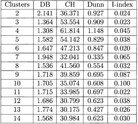
5.2.1 Experimental Results of fc-MCMA 45
5.2.2 Experimental Results of EMMA 47
5.3 Analysis and Discussion 50
5.4 Comparison with Previous Approaches 58
6 C o n c l u s i o n 65
6.1 Summary of Contributions 65
6.2 Future Work 67
B i b l i o g r a p h y 69
I n d e x 75
List of Figures
1 . 1 The steps required in a microarray experiment O
1 . 2 A sample DNA microarray. 4
3 . 1 Unaligned and aligned profiles 2 2
5 . 1 EMMA clusters, S. cerevisiae phases and fc-MCMA clusters 5 6
O . A fc-MCM A clusters and EMMA clusters of P. aeruginosa data set . . . 5 7
O.O S. cerevisiae phases and fc-MCMA clusters using natural cubic spline profiles . . . 5 8
5 . 4 S. cerevisiae phases and fc-MCMA clusters using piecewise linear profiles . . 5 9
5 . 5 EMMA clusters, M. luteus phases and fc-MCM A clusters 6 0
5 . 6 EMMA clusters, S. cerevisiae phases, fc-MCMA clusters, and VCD clusters 6 3
5 . 7 fc-MCMA clusters, EMMA clusters and VCD clusters on S. pombe data set 6 4
List of Tables
1 Declaration of Previous Publications IV
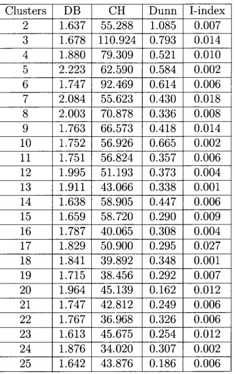
5 . 1 Validity index values for fc-MCMA clusters on the Saccharomyces cerevisiae data set. . . 4 5
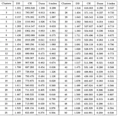
5 . 2 Validity index values for fc-MCMA clusters on the Pseudomonas aeruginosa data set. . . 4 6
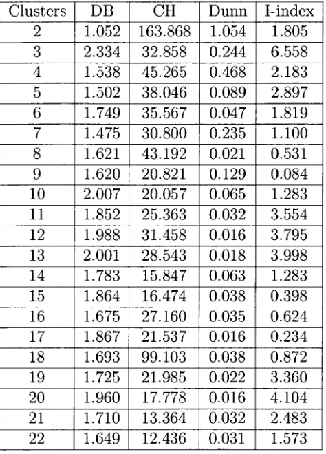
5 . 0 Validity index values for fc-MCMA clusters on the serum data set. . . . 4 7
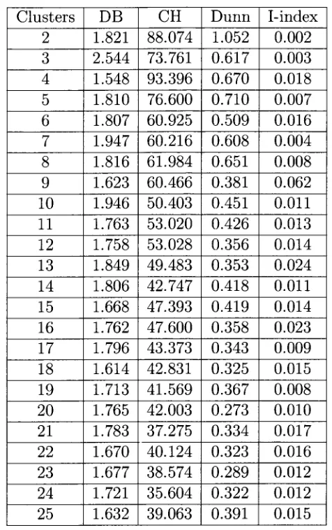
5 . 4 Validity index values for fc-MCMA clusters on the Micrococcus luteus data set. . . . . . 4 8
5 . 5 Validity index values for fc-MCMA clusters on the Escherichia coli data set. . . . . . . 4 9
5 . 6 Validity index values for EMMA clusters on the Saccharomyces cerevisiae data set. . . . 5 0
5 . 7 Validity index values for EMMA clusters on the Pseudomonas aeruginosa data set. . . . 5 1
5 . 8 Validity index values for EMMA clusters on the serum data set 5 2
5 . 9 Validity index values for EMMA clusters on the Micrococcus luteus data set 5 3
5 . 1 0 Validity index values for EMMA clusters on the Escherichia coli data set. . . 5 4
5 . 1 1 Validity index values for EMMA clusters on the Schizosaccharomyces pombe data set. . . 5 5
5 . 1 2 Best number of clusters for all data sets 5 6
5 . 1 3 Experiment results overview of fc-MCMA and EMMA with piecewise linear profile of [15] . 6 1
5 . 1 4 Experiment results overview of EMMA approach and the VCD method of [36] . . . . . 6 2
List of Algorithms
1 k-MCMA: k-Means Clustering with Multiple Alignment . . . . 32
2 EMMA: EM Clustering with Multiple Alignment 36
Chapter 1
Introduction
1.1 Microarray Technology
Micorrarrys are widely used tools in molecular biology providing a fast and
cost-effective method for monitoring the expression of thousands of genes
si-multaneously [30]. Microarrays enable monitoring of whole-genome expression
in a single experiment. The biological interpretation of large datasets is the
biggest challenge for scientists confronted with gene expression data.
A cDNA microarray is an arrayed series of thousands of microscopic spots
of DNAs each containing a specific DNA sequence, known as probe. A probe
can be a short section of a gene or other DNA element that is used to hybridize
a cDNA or cRNA sample, known as target. In oligonucleotide microarrays, the
probes are short sequences designed to match parts of the sequence of known
or predicted open reading frames. Oligonucleotide arrays are produced by
printing short oligonucleotide sequences designed to represent a single gene or
family of gene splice-variants by synthesizing this sequence directly onto the
CHAPTER 1. INTRODUCTION 2
array surface instead of depositing intact sequences. Sequences may be longer
(60-mer probes) or shorter (25-mer probes) depending on the desired
pur-pose; longer probes are more specific to individual target genes, while shorter
probes can be spotted in higher density across the array and are cheaper to be
produced. In spotted microarrays, the probes are oligonucleotides, cDNA or
small fragments of P C R products that correspond to mRNAs. The probes are
synthesized prior to deposition on the array surface and are then "spotted"
onto the glass.
Microarrays are solid substrates hosting hundreds of single stranded DNAs
with a specific sequence. DNA Microarrays are solid supports onto which the
sequences from thousands of different genes are attached at fixed locations.
The supports themselves are usually glass microscope slides, but can be silicon
chips or nylon membranes on which the DNA is printed, spotted or
synthe-sized. The whole microarray technology is based on hybridization probing,
a technique that uses fluorescence labeled nucleic acid molecules as mobile
probes to identify complementary molecules. A typical DNA microarray
ex-periment involves the following steps:
1. Preparing the DNA chip using the chosen targets.
2. Generating hybridization mixture of fluorescence labeled cDNAs.
3. Incubating hybridization mixture with the DNA chip.
4. Detecting bound cDNA using laser technology
CHAPTER 1. INTRODUCTION 3
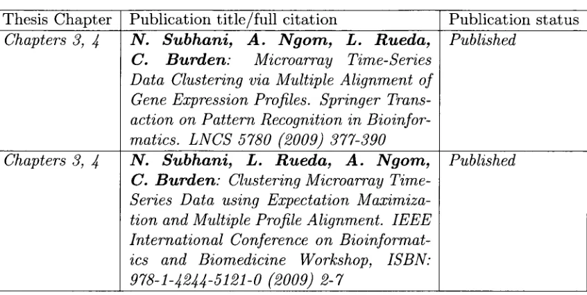
Figure 1.1* illustrates the typical process of a DNA microarray experiment.
:' •s""3 tmi
dm ' •» IT" -i ftM»,"IM«M ilKA ' »->
1dSBB1 MtONA
Purification RT Coupling Hybridization Scanning and washes and analysis
Figure 1.1: T h e steps required in a microarray experiment.
The amount of fluorescence emitted by each cDNA array will be
propor-tional to the amount of mRNA produced from the gene having the
corre-sponding DNA sequence. The above description is for DNA microarrays only
but the microarray experiments vary according to the specific type of
microar-ray. In [23], four main technology platforms of microarrays are described: 1)
Nylon membrane arrays or radioactive filters; 2) cDNA arrays or red/green
arrays; 3) Polynucleotide arrays; 4) Oligonucleotide arrays (also called DNA
chips). cDNA technology is the most commonly used one, and allows spotting
of almost any P C R product. Gene expression levels are detected over a period
of time from microarrays. Then the expression ratio of genes are measured
by using different logarithmic and normalization techniques. These kinds of
gene expressions over a period of time are called time-series gene expression.
Time-series gene expression d a t a can be produced by any of the above
mi-croarrays and even other technologies. We are considering any form of the
technology that produces time-series gene expression data.
CHAPTER 1. INTRODUCTION 4
• * & •>;• • • © * m • «* • * ^ ®
a * • « • ' • « « • ® • * * • «
* • • • ..< • • •
# ® « »• • » > • i- » # »
• B « : « V • • a • • •
0 # # ^ » » • G m #
• a * » •! » ® • • « • • » • • » «s ii t» »: » » • • *> '«' » ' « 'i
is ® • .<• ma :
m m • • :: • »
d :::: . ;.;: « <? V *
a a «
(; ® s • » m m m»
» si « • e
• • « ' 0 0 * « 0 « ^ & &
« » • « • 1' 0 • < ::,:. e t) 0 i • * « • « • s
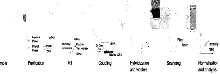
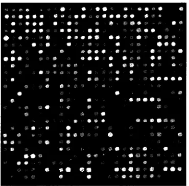
Figure 1.2: A sample D N A microarray.
1.2 Microarray Analysis
Microarray technology has the following important advantages:
1. it can measure the expression levels of thousands of genes in parallel,
2. it provides semi-quantitative data, and
3. it is sensitive enough to detect low-abundance transcripts that are
rep-resented on a given array.
DNA microarrays are used for measuring the concentration of mRNA in living
cells. The concentration of a particular mRNA transcript is measured as the
expression level of its corresponding gene. The expression profile, a snapshot
of the total mRNA pool of living cell or tissue, can be obtained when different
probes matching all mRNAs in a cell are used. It reflects the expression of
every single measured gene at that particular moment. The expression can
also be used to quantify the expression of a single gene over a number of
CHAPTER 1. INTRODUCTION 5
Microarrays have been successfully used in a wide range of applications
including sequencing, SNP detection and cluster analysis. However, the main
application still remains the investigation of the genetic mechanisms in living
cells. The microarray technology has a very high throughput interrogating
thousands of genes at the same time. It has been proved that microarrays can
be used to generate reliable and accurate gene expression data [7, 37]. It can
also be used for purely computational purposes such as in the field of DNA
computing [5].
1.3 Microarray Time-Series Gene Expression
An increasingly popular method for studying a wide range of biological
sys-tems is through time-series expression experiments. In time-series expression
experiments, a snapshot of the expression of genes in a temporal process is
measured rather than in different samples. Another main characteristic of
the time-series data is to exhibit a strong autocorrelation between
succes-sive points rather than from a sample population (which are assumed to be
independent and identically distributed).
Gene expression is a measurement of expressed gene over a certain
pe-riod of times under different conditions. Different proteins are required and
synthesized for different functions, under different conditions and at different
times. One of the most important ways of new protein generation in which
the cell regulates gene expression is by using a feedback loop. In many cases,
the expression program starts by activating a few transcription factors (TF),
con-CHAPTER 1. INTRODUCTION 6
dition. It is necessary to measure a time course of expression experiments in
order to determine the complete set of genes that are expressed under new
conditions.
Much of the early work on analyzing time-series expression experiments
used methods developed for static d a t a [19]. Recently, several new approaches
were presented specially targeting time-series expression d a t a [3, 21, 31, 11,
36]. We are also presenting few new clustering approaches specifically for
time-series gene expression profile analysis in Chapter 3 and 4.
1.4 Motivation and Objective
An important process in functional genomic studies is clustering microarray
time-series data, where genes with similar expression profiles are expected to
be functionally related. A common problem in biology is to partition a set of
experimental d a t a into clusters in such a way that the data points within the
same cluster are highly similar while d a t a points in different clusters are as
dis-similar as possible. Profile alignment clustering is based on deciding upon the
similarity often involves pairwise distance measures of co-expressions.
Clus-tering algorithms that apply a conventional distance (e.g. the Euclidian
dis-tance, correlation coefficient) function normally do not reflect the temporal
d a t a embedded in the expression profiles.
We are proposing new profile alignment approaches to cluster microarray
time-series gene expression profiles. Clustering time-series expression data
with unequal time intervals is a very special problem, as measurements are
CHAPTER 1. INTRODUCTION 7
proposed in [15] takes two features vectors, and produces two new vectors in
such a way that the area between the "aligned" vectors is minimized. The
profile alignment method that takes the length of the intervals between the
time-points into consideration was proposed in [15]. In both [15] and [25],
hierarchical agglomerative clustering is used where the decision rule is based
on the furthest-neighbor or complete linkage distance between two clusters.
T h a t clustering approach performs the pairwise alignment before measuring
the distance between two profiles during each iteration, which slows down the
computational process. Also, piecewise linear representation of gene
expres-sion profile was used which does not reflect the actual representation of the
gene expression.
To reflect the actual representation of the gene expression profiles, we
gen-eralize piecewise linear profiles to natural cubic spline profiles. Taking the
lengths of the time intervals into account is accomplished by means of
ana-lyzing the area between two expression profiles, joined by the corresponding
measurements at subsequent time points. This is equivalent to considering the
sum or average of squared errors between the infinite points in the two lines.
This analysis can be easily achieved by computing the underlying integral,
which is analytically resolved in advance, subsequently avoiding expensive
computations during the clustering process. Our approach allows us to apply
flat clustering such as fc-means, which, though not optimal, provides a fast
and practical solution to the problem. We also apply our approach to the
CHAPTER 1. INTRODUCTION 8
1.5 Contributions
In this thesis, clustering approaches are proposed based on the concept of
Profile-Alignment, for clustering microarray time-series gene expression
pro-files. Our main contributions in this thesis are:
1. Generalize the theoretical results of [15] to any continuously integrable
representation of time-series gene expression profiles. The contributions
are:
a) Piecewise Linear (PL) function to Natural Cubic Spline (NCS)
function representation.
b) Pairwise alignment of NCS functions.
c) Distance between two NCS functions.
d) Analytical solutions of b) and c).
2. Multiple Alignment of NCS representations and of PL representations
of gene expressions time-series profiles. The contributions are:
a) Universal Alignment Theorem: align the profiles such that the
squared error between any two vertically shifted profiles is
mini-mal.
b) Centroid of a cluster: a centroid function, which aim to find
repre-sentative profile of a cluster, defined based on natural cubic spline
profiles.
c) Analytical solutions of a) and b).
CHAPTER 1. INTRODUCTION 9
a) Theoretical results: clustering multiple-aligned d a t a is equivalent
to clustering original data, but is faster when using multiple-aligned
data.
b) Clustering multiple-aligned data using any representation (NCS or
PL):
i. /.-Means clustering via multiple alignment (fc-MCMA): an
al-gorithm that clusters multiple aligned profiles with /c-mcans.
ii. EM clustering via multiple alignment (EMMA): a method that
combines EM and multiple alignment of gene expression
pro-files to cluster microarray time-series data.
iii. Theoretical result: we can cluster with any distance-based
clus-tering method.
c) New measure of clustering accuracy using:
i. Hungarian matching algorithm for clustering-phase assignment.
ii. c-Nearest Neighbor (c-NN) method: combined with cross-validation
and validity indices.
Our major contribution is to use the benefit of alignment method in
combi-nation with any clustering method. Initialization is a major issue in /c-means
and EM methods but we are not interested in improving fc-means or EM
CHAPTER 1. INTRODUCTION 10
1.6 Thesis Organization
The thesis is organized in five chapters. Chapter II provides a survey of
clustering, microarray time-series clustering and clustering with alignment.
Chapters III and IV present the proposed alignment approaches and
clus-tering algorithms, respectively. Chapter V deals with experimental results
and performance analysis, where all proposed approaches are analyzed and
compared to existing methods. Finally, Chapter VI concludes the thesis and
Chapter 2
Microarray Time-Series Data
Clustering
A brief review about clustering and its uses are discussed in this chapter.
Microarray time-series data clustering is also formally defined here. The
liter-ature review of previous works on clustering, and specially microarray
time-series data clustering are discussed in Section 2.3.
2.1 Clustering
Clustering is a multivariate analysis technique used to discover unknown
pat-terns or groups in data. Clustering is appropriate when there is no a priori
knowledge about the underlying data. Clustering, the process of grouping
similar entities, can be done on any data such as genes, samples, time points
in a time-series, etc. The particular type of input makes no difference on the
clustering algorithm. The algorithm will treat all inputs as an n-dimensional
CHAPTER 2. MICROARRAY TIME-SERIES DATA CLUSTERING 12
feature vector. To group objects that are similar, we need a very precise
definition of measure of similarity. There are many different ways in which
such a measure of similarity can be calculated depending on the
representa-tion of gene expression profiles. We are considering clustering on microarray
time-series expression profiles.
2.2 Microarray Time-Series Data Clustering
In this section, we discuss the clustering the problem of the microarray
time-series gene expression profiles. Time-Series clustering problem is formally
stated in order to discuss these approaches. Given a dataset V = ( x i ( t ) , . . . ,
xi = [x%i j • • •, xi„]1 is a n ^-dimensional feature vector that represents the
ex-pression level of gene i at n different time points, t = [£],..., tn]L. We want to
partition a set of s profiles, T>, into k disjoint clusters Ci,..., Ch, 1 < k < s;
such that (i) Ct ± 0,« = 1 , . . . , k; (ii) U.tA = V (iii) C{ n Cj = i ± j ;
i,j = 1 ,...,k. Also, each profile is assigned to the cluster whose distance
is the closest. We are considering the specific case of time-series clustering,
where the order of time-points cannot be permuted because of the different
permutations give different results which are biologically meaningless.
2.3 Literature Review
Many clustering methods for time-series gene expression d a t a have been
de-veloped. A partitional clustering method based on A;-means applied in [29]
CHAPTER 2. MICROARRAY TIME-SERIES DATA CLUSTERING 13
prior knowledge, except the value of k needs to be known a priori, about the
structure or to make any assumptions about the dynamics of the expression
profile. In [20], Tamayo et al applied Self-organizing maps (SOM) to visualize
and interpret the patterns of gene temporal expression profiles. The SOM, a
type of mathemetical cluster analysis suits well with exploratory analysis of
the data and to reveal relevant patterns in a large, high-dimensional dataset.
Several other methods also have proposed including a jack-knife correlation
coefficient model [14], an order-restricted inference-based method [28], a
sta-tistical two-regression step approach [1], a method for assigning genes to
pre-defined set of model profiles [12], and combined spline smoothing and first
derivative computation [27]. In [6], fuzzy clustering of time-series data based
on the similarity of relative change of expression level and the corresponding
temporal information of the profiles.
A hidden phase model was used for clustering time-series d a t a to define
the parameters of a mixture of normal distributions in a Bayesian-like manner
that are estimated by using expectation maximization (EM) [4], A Bayesian
approach in [16], partitional clustering based on /c-means in [29] and an
Eu-clidean distance approach in [20] have been proposed for clustering time-series
gene expression profiles. They have applied self-organizing maps (SOMs) to
visualize and interpret gene temporal expression profile patterns. Also, the
methods proposed in [14, 26] are based on correlation measures. A method
t h a t uses jack-knife correlation with or without using seeded candidate profiles
was proposed for clustering time-series microarray data as well [14]. Specifying
expression levels for the candidate profiles in advance for these
CHAPTER 2. MICROARRAY TIME-SERIES DATA CLUSTERING 14
using a small sample of arbitrarily selected genes. The resulting clusters
de-pend upon the initially chosen template genes, because there is a possibility
of missing important genes. A regression-based method, which is suitable for
analyzing single or multiple microarrays was proposed in [12] to address the
challenges in clustering short time-series expression datasets.
A Bayesian approach for improving the clustering results of gene expression
series using rough knowledge the general shapes of the classes was proposed
[4]. Knowledge about the general shapes can be elementary regarding the
change of the mean expression level over time. The information regarding the
shape of the class are directly integrated into the model so that class with the
desired profiles are favored. A Bayesian method was also applied for
model-based clustering where the models are autoregressive curves of fixed order
[16]. To search for the most likely set of clusters out of the given temporal
expression data, an agglomerative procedure was used. The dynamic nature of
gene expression time-series data explicitly takes into account during clustering.
This approach also identifies the number of distinct clusters based on the
well-known Akaike information criterion. This approach is a specialized version of
Bayesian Clustering by Dynamics where two time-series are considered similar
if they are generated by the same stochastic process.
In [28], Peddada et al. applied an order-restricted inference method for
se-lecting and clustering genes expression profiles for time-series or dose-response
data. The method applies the ideas of order-restricted inference and uses
known inequalities among parameters. In this procedure, two profiles are
placed in the same cluster only if all the inequalities between the expected
CHAPTER 2. MICROARRAY TIME-SERIES DATA CLUSTERING 15
use of the ordering in a time-series study and can detect genes more
sen-sitively using their temporal ordering and finding consistent patterns over
time. A regression-based approach t h a t identifies genes with different
expres-sion profiles across analytical groups in time-series experiments was proposed
in [lj.This method uses a two-step regression strategy, where the first step
adjusts a global regression model with all the defined variables to identify
differentially expressed genes and the next step finds statistically-significant
different profiles by applying a variable selection strategy t h a t studies the
difference between the groups. This method can be used to find genes with
significant temporal expression changes between experimental groups, and to
analyze the magnitude of these differences.
The analysis of gene temporal expression profiles with the problem of
miss-ing values and non-uniformly sampled data was discussed in [38]. Each
ex-pression profile estimated from observed d a t a where gene temporal exex-pression
profiles are represented as continuous curve using statistical spline estimation.
The spline coefficients of the genes are constrained in such way that similar
expression patterns fall into the same class. In [27], a method that focuses
on the shapes of the curves and not on the absolute levels of expression was
proposed to obtain relevant clustering of gene expression temporal profiles by
identifying homogeneous clusters of genes. It combines first derivative
com-putations and spline smoothing with hierarchical and partitional clustering.
This approach is based on the framework of functional d a t a analysis [24],
which focuses on the first derivative of curves by means of a priori spline
smoothing.
CHAPTER 2. MICROARRAY TIME-SERIES DATA CLUSTERING 16
level rate of change across time-points was proposed in [6]. The similarity
between gene expression time-series profiles was calculated by measuring the
difference of the slopes between the functions, where gene temporal profiles
were represented as piece-wise linear functions. The variable time intervals
are viewed as weights, where far apart expressions take smaller weights in the
comparison. A clustering algorithm was proposed which is motivated by the
advantages of fuzzy clustering, and incorporates the distance measure in the
fuzzy-c-means clustering scheme [10].
Clustering based on profile alignment has been discussed recently [3, 21,
31, 11, 36]. In [36], the authors proposed an approach t h a t translates gene
expression into gene variation vectors and derives the proximity measure for
these vectors. In [3], the authors proposed a method t h a t finds clusters of
genes such that the genes within a cluster share a common alignment, but
each cluster is aligned independently of the others. The authors also present
a segment-based alignment algorithm for time series. A clustering method
that uses a local shape-based similarity measure based on Spearman rank
correlation is proposed in [21]. In their method, similar local regions can be
time-shifted to allow the detection of transcription control relationships. An
alignment method that uses HMMs to align time-series gene expression to a
common profile has been introduced in [31]. An Area-based profile alignment
and mean-square-error profile alignment methods have been introduced in [15]
Chapter 3
Gene Expression Profile Alignment
Methods
Many clustering methods have been developed, and each has its own
advan-tages and disadvanadvan-tages regarding handling noise in the measurements and
the properties of the data set being clustered. In [15], hierarchical clustering
was used and the decision rule was the farthest-neighbor distance between two
clusters computed using an equivalent of Eq. (3.1) for piece-wise linear
pro-files. Hierarchial clustering is a greedy method that cannot be readily applied
on large data sets.
An important process in functional genomic studies is clustering
microar-ray time-series data, where genes with similar expression profiles are expected
to be functionally related. A common problem in biology is to partition a
set of experimental data into clusters in such a way that the data points
within the same cluster are highly similar while data points in different
clus-ters are as dissimilar as possible. Profile alignment clustering is based on
CHAPTER 3. GENE EXPRESSION PROFILE ALIGNMENT METHODS 18
deciding upon the similarity often involves pairwise distance measures of
co-expressions. Clustering algorithms t h a t apply a conventional distance (e.g.
the Euclidian distance, correlation coefficient) function normally do not
re-flect the temporal data embedded in the expression profiles. We are proposing
new profile alignment approaches to cluster microarray time-series gene
ex-pression profiles.
3.1 Clustering with Alignment
There is some alignment techniques already introduced to resolve this issue
before applying the distance function. Area based profile alignment proposed
in [15] takes two features vectors, and produces two new vectors in such a way
that the area between "aligned" vectors is minimized. The profile alignment
method that takes the length of the intervals between the time-points into
con-sideration was proposed in [15]. T h a t approach considers the weights of the
intervals equally, irrespective to the actual size of the interval of the
measure-ment. The Profile-Alignment algorithm takes two feature vectors from the
original space as input and outputs two feature vectors in the transformed
space after aligning them in such way that the sum of squared errors is
min-imized. The alignment of the profiles is done using an area-based distance
function rather than conventional distance functions. The area-based
dis-tance function is defined by computing the integral disdis-tance between the two
aligned profiles. In both [15] and [25], hierarchical agglomerative clustering is
used where the decision rule is based on the furthest-neighbor or complete
CHAPTER 3. GENE EXPRESSION PROFILE ALIGNMENT METHODS 19
approach calculates the distance between the furthest pair of points for each
pair of clusters and merges the two clusters that have the minimum distance
among all such distances between all pair of clusters under consideration. T h a t
clustering approach does the pairwise alignment before measuring distance
be-tween two profiles during each iteration, which slows down the computational
process. Also piecewise linear representation of gene expression profile does
not reflect the actual representation of the gene expression.
We re-formulate the profile alignment problem of [15] in terms of
inte-grals of arbitrary functions, allowing us to generalize from a piecewise linear
interpolation to any type of interpolation one believes be more physically
realistic. The expression measurements are basically snapshots taken at
time-points chosen by the experimental biologist. The cells expressing genes do not
know when the biologist is going to choose to measure gene expression, which
one would guess is changing continuously and smoothly at all the time points.
Thus, smooth spline curve through the known time-points in the cell's
expres-sion path would be a better guess. We use natural cubic spline interpolation
to represent each gene expression profile, which gives a handy way to align
profiles for which measurements were not taken at the same time-points. We
generalize the pairwise expression profile alignment formulae of [15] from the
case of piece-wise linear profiles to profiles which are any continuous integrable
function on a finite interval. Next, we extend the concept of pairwise
align-ment to multiple expression profile alignalign-ment, where the profiles from a given
set are aligned in such a way that the sum of squared errors over a time-interval
defined on the set is minimized. Finally, we combine A;-rrieans clustering with
CHAPTER 3. GENE EXPRESSION PROFILE ALIGNMENT METHODS 20
this thesis, we call this clustering approach as k-Means Clustering via
Multi-ple Alignment (fc-MCMA). Our multiMulti-ple alignment approach is also combined
with expectation-maximization (EM) clustering, called as EM Clustering via
Multiple Alignment (EMMA) to cluster microarray time-series data.
3.2 Alignment Methods for Continuous and
In-t e g r a In-t e FuncIn-tions
3.2.1 Pairwise Alignment
Given two profiles, x(t) and y(t) (either piece-wise linear or continuously
in-tegrable functions), where y(t) is to be aligned to x(t), the basic idea of
align-ment is to vertically shift y(t) towards x(t) in such a way that the squared
errors between the two profiles is minimal. Let y(t) be the result of shifting
y(t). Here, the error is defined in terms of the areas between x(t) and y(t)
in interval [0, T]. Functions x(t) and y(t) may cross each other many times,
but we want that the sum of all the areas where x(t) is above y(t) minus the
sum of those areas where y(t) is above x(t) to be minimal (see Fig. 3.1). Let
a denote the amount of vertical shifting of y(t). Then, we want to find the
value amjn of a that minimizes the integrated squared error between x(t) and
y(t). Once we obtain am;n, the alignment process consists of performing the
shift on y{t) as y(t) = y(t) - am i n.
The pairwise alignment results of [15] generalize from the case of piece-wise
linear profiles to profiles which are any integrable functions on a finite interval.
CHAPTER 3. GENE EXPRESSION PROFILE ALIGNMENT METHODS 21
The alignment process consists of finding the value a that minimizes
rT r . , 9 cT
fa(x(t),y(t))= [ \x(t)-y(t)]2dt= [ \x(t) - [y(t) - a]
Jo 1 J Jo L J
Differentiating yields
dt. (3.1)
A
da" fa(x(t),y(t)) = 2 [ \x(t)+a-y(t)]dt = 2 [ \x{t)-y(t) Jo 1 J Jo 1
dt + 2aT. (3.2)
Setting j-fa(x(t), y(t)) = 0 and solving for a gives
1 fT r n
Omin = -Tp J x(t)-y(t) dt, (3.3)
and since j^fa(x(t),y(t)) = 2T > 0 then amin is a minimum. The integrated
error between x(t) and the shifted y(t) = y(t) — amjn is then
[ \x(t) - y(t)]dt = f \x(t)-y(t)
Jo J Jo L J
dt + aminT = 0. (3.4)
In terms of Fig. 3.1, this means that the sum of all the areas where x(t)
is above y(t) minus the sum of those areas where y(t) is above x(t) is zero.
Given an original profile x{t) = [ei, e 2 , . . . , e„] (with n expression values
taken at n time-points t\, t2, • •., tn), we use natural cubic spline interpolation,
with n knots, (tl 5 e i ) , . . . , (tn, en), to represent x(t) as a continuously integrable
function
xi{t) if ti <t<t2
x(t) = ; (3.5)
xn-i(t) if tn_i<t<tn
where Xj(t) = Xj3(t — tj)3 + Xj2(t — tj)2 + x3] (t — tj)1 + x]()(t — tj)° interpolates
x(t) in interval [tj,tj+1], with spline coefficients Xjk € for 1 < j < n — 1
CHAPTER 3. GENE EXPRESSION PROFILE ALIGNMENT METHODS 22
For practical purposes, given the coefficients, Xjk £ 5?, associated with
x(t) = [ei, e2, . . . , en] € 3?n, we need only to transform x(t) into a new space as
x{t) = [xi3, X12, Xn, Xio, • . • , Xj3, Xj2, Xji, Xjo, . . . , X(n-1)3) £(n-l)2? X(„_i)x, G
gfj4(n_1). We can add or subtract polynomials given their coefficients, and the
polynomials are continuously differentiable. This yields an analytical solution
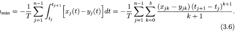
for omin in Eq. (3.3) as follows:
— - 4 e r h'> - » « ] * - - f £ t
j=1 J ti j=1 fc=0
(3.6)
Fig. 3.1(b) shows a pairwise alignment, of the two initial profiles in Fig.
3.1(a), after applying the vertical shift y(t) y(t) — amjn. The two aligned
profiles cross each other many times, but the integrated error, Eq. (3.4), is
zero.
Figure 3.1: (a) Unaligned, and (b) Aligned profiles x(t) and y(t) after applying y(t) y(t) — amjn.
In particular, from Eq. (3.4), the horizontal t-axis will bisect a profile x(t)
CHAPTER 3. GENE EXPRESSION PROFILE ALIGNMENT METHODS 23
section, we use this property of Eq. (3.4) to define the multiple alignment of
a set of profiles.
3.2.2 Multiple Alignment
Given a set D — { x i ( £ ) , . . . , xs(t)}, we want to align the profiles such t h a t the
integrated squared error between any two vertically shifted profiles is minimal.
Thus, for any Xi(t) and x3(t), we want to find the values of ar and a3 that
minimize
rT „ o rT
f r i2 f i
fai,a, (xi(t),xj(t)) =
/
Xi(t)-Xj(t) dt =I
[xi
(t)
-
Oi]-[xj
{t)
- aj]
Jo 1 • ' J o 1
2
dt,
(3.7)
where both Xi(t) and Xj(t) are shifted vertically by an amount a; and a3,
re-spectively, in possibly different directions, whereas in the pairwise alignment
of Eq. (3.1), profile y(t) is shifted towards a fixed profile x(t). The
mul-tiple alignment process consists then of finding the values of ai,... ,as t h a t
minimize
Fai_a,(x1(t),...,xa(t))= (3-8)
l<i<j<s
We use Lemma 3.2.1 to find the values aj and aj, 1 < i < j < s, that
minimize Fa^,„A s.
L e m m a 3.2.1. If Xi(t) and Xj(t) are pairwise aligned each to a fixed profile,
z(t), then the integrated error JQT [Xi(t) — Xj(t)] dt = 0.
Proof. If Xi(t) and Xj(t) are pairwise aligned each to z(t), then from Eq. (3.3),
we have am i n i = /QT [z(t) - Xi(t)] dt and am i n. = JQT [z(t) - Xj(t)] dt.
CHAPTER 3. GENE EXPRESSION PROFILE ALIGNMENT METHODS 24
So [Xi(t) - Xj(t)] dt = Jq [[Xj(£) - am i nJ - [Xj(t) - am i nJ ] dt =
J0T Xi(t)dt + f0T [z(t) - Xi(t)] dt - f0T Xj(t)dt - J0T [z(t) - xj(t)} dt = 0. •
In other words, Xj(t) is automatically aligned relative to .x?(i), given z(t)
is fixed.
Corollary 3.2.2. I f x ^ t ) andxj(t) are pairwise aligned each to a fixed profile,
z(t), then famin.,aminj (xi(t),xj(t)) is minimal.
Proof. From Lemma 3.2.1,
So &(<) - Xj(t)] dt = 0 /0 T [[xi(t) - am i nJ - [xj(t) - am i nJ ]2 dt is minimal.
•
L e m m a 3.2.3. If profiles X \ ( t ) , . . . , xs( t ) are pairwise aligned each to a fixed
profile, z ( t ) , then FaaiBii...,amSnB { xx( t ) , . . . , xa( t ) ) is minimal.
Proof. From Corollary 3.2.2, fauaj ( x i { t ) , x j ( t ) ) > f a ^ a ^ . {xi(t),Xj(t)), with
equality holding when a^ = aminfc; which is attained by aligning each Xk(t)
in-dependently with z(t), 1 < k < s. From the definition of Eq. (3.8), it
follows t h a t Faij...,0s (x1(t),...,xa(t)) > E l < i < j <s /amini ,amin. (Xi(t), Xj (t)) =
Famini,...,amins (xi(t),...,xa(t)), with equality holding when ak = amink, 1 <
k<s. •
Thus, given a fixed profile z(t), applying Corollary 3.2.2 to all pairs of
profiles minimizes Faii...)0s ( x i ( t ) , . . . , xs( t ) ) in Eq. (3.8).
T h e o r e m 3.2.4. Given a fixed profile, z(t), and a set of profiles, X =
CHAPTER 3. GENE EXPRESSION PROFILE ALIGNMENT METHODS 25
such that
1 F \ 1 Xi(t) = Xi(t) - am i n i, where, am i n i = - — J \z(t) - Xi(t) dt, (3.9)
and, in particular, for profile z(t) = 0, defined by the horizontal t-axis, we
have
1 fT
Xi(t) = Xi(t) - om i n i, where, am i n. = — J Xi(t)dt. (3.10)
We use the multiple alignment of Eq. (3.10) in all subsequent discussions.
Using spline interpolations, each profile Xi(t), 1 < i < s, is a continuously
integrable profile
xi,l(f) if tx < t < h
Xi(t) = < (3.11)
xi,n-l(t) if 1 < t < tn
where, xi,j(t) = Xijz(t — tj)z + Xij2(t — tj)2-\-xiji(t — tj)1 +Xij0(t — tj)° represents Xi(t) in interval [t,3, tJ+1], with spline coefficients xl?i, for 1 < i < s, 1 < j <
n — 1 and 0 < k < 3. Thus the analytical solution for am;n i in Eq. (3.10) is
n-1 3 I h J. XJ
run* — Tf, xijk {tj-1-1 t j )
k+1
j=1 fc=0 k + 1
(3.12)
3.2.3 Distance Function
The distance between any two piecewise linear profiles was defined as / ( amin)
in [15]. For convenience here, we change the definition slightly to:
rT i i / r
CHAPTER 3. GENE EXPRESSION PROFILE ALIGNMENT METHODS 26
For any function 4>(t) defined on [0,T], we also define
Then, from Eqs. (3.1) and (3.3),
i rT r
d(x, y) = ^J [[x(t) - y(t)}2 + 2amin [x(t) - y(t)) +
i fT r l2
= T J0 ~ ^ J d t ~ 2a™in + a™in
(3.14)
dt
= ([x{t) - y{t)}2) - (x(t)-y{t)}2. (3.15)
Apart from the factor this is precisely the distance dpA.{x,y,t) in [15].
By performing the multiple alignment of Eq. (3.10) to obtain new profiles
x(t) and y(t), we have:
fT
d(x, y) = ([x(t) - y(t)]2) = f j [£(*) - Vit) dt. (3.16)
Thus, d(x, y)^ is the 2-norm, satisfying all the properties we might want for
a metric. On the other hand, it is easy to show that d(x, y) in Eq. (3.16) does
not satisfy the triangle inequality, and hence it is not a metric. We, however,
use d(x,y) in Eq. (3.16) as our distance function, since it is algebraically
easier to work with than the metric d(x, y)^. Eq. (3.16) is closer to the spirit
of regression analysis, and thus, we can dispense with the requirement for the
triangle inequality. Also the distance as defined in Eq. (3.16) is unchanged
by an additive shift, and hence, is order-preserving; t h a t is: d(u, v) < d(x, y)
if and only if d (u, v) < d (x. y). This property has important implications for
distance-based clustering methods that rely on pairwise alignments of profiles;
CHAPTER 3. GENE EXPRESSION PROFILE ALIGNMENT METHODS 27
With the spline interpolations of Eq. (3.5), we derived the analytical solution for d{x,y) in Eq. (3.16), using the symbolic computational package, Maple*, as follows:
P2(n7 — m7) (2PQ - 6P2m)(n6 - m6) (2PR - 10PQm + Q2 + 15P2m2)(n5 - m5)
d(x, y) — + -| -
|-7 6 5 ( - 8 P R m - 4Q2m + 2PS + 20PQm2 + 2QR - 20P2m3)(n4 - m4)
4
(-6QRm - 20Pm3Q + R2 + 6Q2m2 + 12Pm2R - 6PmS + 15P2m4 + 2Q5)(n3 - m3)
{
3
(10Pm4<3 + 6Qm2R + 2RS - 8Pm3R - 2R2m - 6P2m5 + &Pm2S - 4QmS - 4Q2m3)
(n2 - m2)} - 2RmS(n - m) + S2(n - m ) + P2m6(n - m ) + Q2mA[n - m) +
R2m2(n - m) - 2Qm3R(n - m) - 2Pm5Q(n - m) - 2Pm3S(n - m) +
2Pm4R(n - m) + 2Qm2S(n - m) (3.17)
where P = (xj3 - yj3), Q = (xj2 - R = {xji - Vji), S = (xj0 - yj0 +
cy — cx)i m = tj and n = tj+\.
3.2.4 Centroid of a Cluster
Given a set of profiles D = ( x i ( t ) , . . . , rcs(i)}, we aim to find a centroid profile
fi(t) that well represents D. An obvious choice is the function that minimizes
s
= (3.18) i=i
where A plays the role of the within-cluster-scatter defined in [15]. Since d(-, •)
is unchanged by an additive shift x(t) x(t) — a in either of its arguments,
we have
s 1 fT S
A\ii) = Y , d { xi, n ) = - I (3.19)
2 = 1 i= 1
where, X = {xi(t),..., xs(t)} is the multiple alignment of Eq. (3.10). This
is a functional of /x; that is, a mapping from the set of real valued functions
CHAPTER 3. GENE EXPRESSION PROFILE ALIGNMENT METHODS 28
defined on [0, T] to the set of real numbers. To minimize with respect to /i we
set the functional derivative to zero*. This functional is of the form
F[<j>] = J L(<j>(t))dt, (3.20)
for some function L, for which the functional derivative is simply
6<p(t)
• In our case, we have
5A[/x] 2 &(*) - Hit)] = -7r E Xi{t) - sn(t) . (3.21) > i=l \ i = l
Setting = o gives
1 s
V(t) = - ^ X i i t ) . (3.22) s
2 = 1
With the spline coefficients, of each Xi(t) interpolated as in Eq. (3.11),
the analytical solution for /j,(t) in Eq. (3.22) is
3
2 = 1
] xijk (t t j )
,k=0
— am;n i, in each interval [tj,tj+i]. (3.23)
Eq. (3.22) applies to aligned profiles while Eq. (3.23) can apply to unaligned
profiles.
3.3 Alignment Methods for Piecewise Linear
Func-tions
In this chapter, we have proposed pairwise alignment, multiple alignment,
distance function and centroid of a cluster for continuous integrable functions
^For a functional F [<-/;], the functional derivative is defined as ^(tj =
CHAPTER 3. GENE EXPRESSION PROFILE ALIGNMENT METHODS 29
which is Natural Cubic Spline function. All the above theoretical results on
Natural Cubic Spline representations including lemmas and theorems are also
apply to Piecewise Linear representations of time-series profiles. Clustering
algorithms that are proposed in the next chapter also apply to Piecewise
Chapter 4
Clustering via Continuous Gene
Expression Profile Alignment
In both [15] and [25], profiles were represented as piecewise linear functions.
Area-based profile alignment takes two features vectors, and produces two new
vectors in such a way that the area between "aligned" vectors is minimized.
In [15], hierarchical-agglomerative-clustering is used where the decision rule
is based on the furthest-neighbor or complete linkage distance between two
clusters. The complete linkage or furthest neighbors calculates the distance
between the furthest pair of points for each pair of clusters and merges the two
clusters that have the minimum distance among all such distances between
all pairs of clusters under consideration. The proposed clustering algorithms
are discussed in this chapter. Validity indices to determine the accuracies of
the proposed approaches and to determine the number of clusters are also
discussed.
CHAPTER 4. CLUSTERING VIA CONTINUOUS GENE EXPRESSION
PROFILE ALIGNMENT 31
4.1 £;-Means Clustering via Multiple Alignment
The fc-means algorithm is one of the simplest and fastest clustering algorithms.
It takes the number of clusters, k, as an input parameter. The program starts
by randomly choosing k points as the centers of the clusters. These points
may be just random points from more densely populated volumes of the input
space or just randomly chosen patterns from the data itself. Once some cluster
centers have been chosen, the algorithm will take each profile and calculate
the distance from it to all cluster centers. Since the cluster centers were
chosen randomly, it is not said t h a t this is the correct clustering. The second
steps starts by considering all profiles associated which one cluster center and
calculating a new position for this cluster center. The coordinates of this
new center are usually obtained by calculating the mean of the coordinates
of the points belonging to that cluster. Since the centers have moved, the
profile memberships need to be updated by recalculating the distance from
each profile to the new cluster centers. The algorithm continues to update
the cluster centers based on the new membership and update the membership
of each profile until the cluster centers are such that no profile moves from
one cluster to another. Since no profile has changed its membership, the
centers will remain the same and the algorithm will terminate. A more formal
definition of /e-means clustering is stated below.
In A;-means [35], we want to partition a set of s profiles, T> — {x\(t),..., xs(£)},
into k disjoint clusters Ci,..., C/., 1 < k < s; such that (i) Ci ^ 0, i = 1 , . . . , k\
(ii) Uf=lCi = V (iii) Ci fl Cj = i j^ j; i,j = 1 ,...,k. Also, each profile
CHAPTER 4. CLUSTERING VIA CONTINUOUS GENE EXPRESSION
PROFILE ALIGNMENT 32
mixtures of Gaussians in the sense that they both attempt to find the centers
of natural clusters in the data. It assumes that the object features form a
vector space. Let U = {uVJ} be the membership matrix defined as follows:
{ 1 if d (xi, fij) = mini=i i-d (x,, jii) where i = l,...,s (4.1) 0 otherwise
The aim of fc-means is to minimize the sum of squared distances:
n k
= (4-2)
%=i j=i
where 0 = //i,/x2,
A l g o r i t h m 1 k-MCMA: k-Means Clustering with Multiple Alignment Input: Set of profiles, T> — {xi(t),... ,xs(t)}, and desired number of clusters,
k
O u t p u t : Clusters C^,..., Cp,k
1. Apply natural cubic spline interpolation on xi(t) G T>, for 1 < i < k (see Section 3.2.1)
2. Multiple-align transformed T> to obtain T> = { x i ( t ) , . . . , using Eq. (3.10)
3. Randomly initialize centroid p>i(t), for 1 < i < k
r e p e a t
4.a. Assign Xj(t) to cluster CIH with minimal d (x3, fij), for 1 < j < s and
1 <i<k
4.b. Update /tj(£) of C^, for 1 < i < k
until Convergence: t h a t is, no change in fii(t), for 1 < i < k r e t u r n Clusters C ^ , . . . , Cp,k
In A-MCMA (see Algorithm. 1), we first multiple-align the set of profiles
V, using Eq. (3.10), and then cluster the multiple aligned V with fc-means.
Recall that the process of Eq. (3.10) is to pairwise align each profile with
CHAPTER 4. CLUSTERING VIA CONTINUOUS GENE EXPRESSION
PROFILE ALIGNMENT 33
profiles in t>, and then take the centroid of each pair. In step (4.a), we do
not use pairwise alignment to find the centroid [ii{t) closest to Xj(t), since,
by Lemma 3.2.1, they are automatically aligned relative to each other. When
profiles are multiple-aligned, any arbitrary distance function other than Eq.
(3.16) can be used in step (4.a), including the Euclidean distance. Also, by
Theorem 4.1.1 below, there is no need to multiple-align C^ in step (4.b), to
update its centroid fiiit).
T h e o r e m 4.1.1. Let jl(t) be the centroid of a cluster of m multiple-aligned
profiles. Then p,(t) = fl(t).
Proof. We have p,(t) = p,(t) - am i n- . However, am i n- = ^ JQT p,(t)dt
= T Jo m i = since each Xi(t) is aligned with the £-axis. • •
Thus, Lemma 3.2.1 and Theorem 4.1.1 make fc-MCMA much faster than
applying fc-means directly on the non-aligned dataset T>, and even more than
this when the Euclidean distance is used to assign a profile to a cluster. An
important implication of Eq. (3.16) is t h a t applying fc-means on the
non-aligned dataset V (i.e., clustering on £>), without any multiple alignment,
is equivalent to fc-MCMA (i.e., clustering on T>). T h a t is, if a profile xi(t)
is assigned to a cluster CIH by fc-means on T>, its shifted profile Xi{t) will
be assigned to cluster C^ by fc-MCMA (fc-means on T>). This can be easily
shown by the fact that multiple alignment is order-preserving, as pointed out
in Section 3.2.3. In fc-means on Z>, step (4.a) would require 0{sk) pairwise
alignments to assign s profiles to fc clusters, whereas no pairwise alignment is
needed in fc-MCMA. In other words, we show that we can multiple-align once,
CHAPTER 4. CLUSTERING VIA CONTINUOUS GENE EXPRESSION
PROFILE ALIGNMENT 34
means in the same manner. This also reinforces a known fact demonstrated in
[33], which is a dissimilarity function that is not metric can be made metric by
using a shift operation (in our case any metric can be used in step (4.a) such as
the Euclidean distance). In this case, the objective function of A;-means does
not change, and convergence is assured. Thus, this saves a lot of computations
and opens the door for applications of multiple alignment methods to many
distance-based clustering methods.
4.2 E M Clustering via Multiple Alignment
In [18], we devised a clustering approach, A-MCMA, where we combined the
multiple alignment of Eq. (3.10) and the A;-means clustering method with
a distance function based on the pairwise alignment of Eq. (3.3). In this
section, we use the EM clustering algorithm instead and combine it with the
alignment methods.
EM is used for clustering in the context of mixture models [2], The goal
of EM clustering is to estimate the means and standard deviations for each
cluster so as to maximize the likelihood of the observed d a t a (distribution).
In other words, the EM algorithm attempts to approximate the observed
distributions of values based on mixtures of different distributions in different
clusters. A mixture of Gaussians is a set of k probability distributions, where
each distribution represents a cluster. With an initial approximation of the
cluster parameters, it iteratively performs two steps: first, the expectation step
computes the values expected for the cluster probabilities, and second, the
CHAPTER 4. CLUSTERING VIA CONTINUOUS GENE EXPRESSION
PROFILE ALIGNMENT 35
until the log-likelihood reaches a (possibly local) maximum. The algorithm is
similar to fc-means in the sense that the centers of the natural clusters in the
data are re-computed until a desired convergence is achieved.
In EM [35], we want to partition a set of s profiles, V = {xi(t),..., xs(t)},
into k disjoint clusters Ci,..., C 1 < k < s, such that; (i) Q ^ 0, i = 1 , . . . , A;;
(ii) U=ici = ^ (i") CiHCj = = 1 ,...,k and i ± j. Let V be the
complete-data space drawn independently from the mixture density:
k
E - s t e p : p(x\6) = \CU 6i)P{Ci) (4.3)
i=1
where parameter 6 = [ 6 \ , . . . , O^}1 is fixed but unknown, and P{Ci) is the known
posterior probability of class Ci. The aim is to maximize the likelihood:
s
M - s t e p : p(D\0) = J J p ( ze| 0 ) (4.4)
e = l
To maximize the likelihood function, log-likelihood is used in the normal
dis-tribution of the component densities given by: p(xk\Ci,9i) ~ Niji.^ £ j ) where
0, = [/ij, Ej]4; /ii and Ei are the means and the covariances of the classes,
respectively. Both steps iterate until the log-likelihood reaches a maximum.
Thus, EM assigns profiles to multiple clusters, like in fuzzy clustering. Also,
unlike in /c-means, each profile is assigned to the cluster that finds the
maxi-mum posterior probability.
In EMMA (see Algorithm 2), we first multiple-align the set of profiles T>,
using Eq. (3.10), and then cluster the multiple-aligned V with EM. Recall
that the process of Eq. (3.10) is to pairwise align each profile with the
t-axis. The k centroids can be initialized randomly in step (3) of EMMA, or by