Analysis of Gene Expression Microarray Time Series Data

A

G

E

M

T

S

D

Ola ElBakry

A Thesis

in

The Department

of

Electrical and Computer Engineering

Presented in Partial Fulfillment of the Requirements

for the Degree of Doctor of Philosophy at

Concordia University

Montreal, Quebec, Canada

April 2013

© Ola ElBakry, 2013

CONCORDIA UNIVERSITY SCHOOL OF GRADUATE STUDIES

This is to certify that the thesis prepared

By: Ola El Bakry

Entitled: Analysis of Gene Expression Microarray Time Series Data

and submitted in partial fulfillment of the requirements for the degree of

DOCTOR OF PHILOSOPHY (Electrical and Computer Engineering)

complies with the regulations of the University and meets the accepted standards with respect to originality and quality.

Signed by the final examining committee:

Chair Dr. P. Grogono External Examiner Dr. E.R.M. Tillier External to Program Dr. R. Ganesan Examiner Dr. W.E. Lynch Examiner Dr. W. Zhu Thesis Co-Supervisor Dr. M.O. Ahmad Thesis Co-Supervisor Dr. M.N.S. Swamy Approved by Dr. J.X. Zhang, Graduate Program Director

April 25, 2013

Dr. Robin Drew, Dean

iii

Abstract

ANALYSIS OF GENE EXPRESSION MICROARRAY TIME SERIES DATA

Ola ElBakry, Ph.D.

Concordia University, 2013.

Regulatory interactions among genes and gene products are dynamic processes, and hence, modeling these processes is essential. In recent years, research efforts in the field of microarray data analysis have been constantly increasing due to the rapid growth of microarray technology, and due to the growing interest in the understanding of complex diseases. It is of vital importance to identify and characterize changes in gene expression over time. Since genes work in a cascade of networks, reconstruction of gene regulatory networks is a crucial process for a thorough understanding of the underlying biological interactions. Analysis of large scale microarray data is a challenging problem, where most of the microarray time series have only five to ten time points and the conventional time analysis techniques are not applicable.

The present study focuses on two important aspects of the microarray data analysis. The first part is concerned with the identification of the differentially expressed genes, whereas the second part with the reconstruction of the gene regulatory networks. New computational methods for time course microarray data that assist in analyzing and modeling the dynamics of the gene regulations are developed in this study.

The main challenges in the identification of differently expressed genes arise due to the availability of a very small number of replicated samples (usually two or three samples) in the face of a huge number of genes (thousands of genes). Further, most of the previous works, in this area have focused on static gene expressions, with only a limited number on methods for selecting the genes that exhibit changes with time. In the first part of this study, a general statistical method for detecting changes in microarray expression over time within a single or

iv

multiple biological groups is presented. The method is based on repeated measures (RM) ANOVA, in which, unlike the classical F-statistic, statistical significance is determined by taking into account the time dependency of the microarray data. A correction factor for this RM F-statistic that leads to higher sensitivity as well as a high specificity is introduced. The two approaches for calculating the p-values that exist in the literature, that is, those resampling techniques of gene-wise p-values and pooled p-values, are investigated. It is shown that the pooled p-values method compared to the method of the gene-wise p-values is more powerful and computationally less expensive, and hence it is applied along with the correction factor introduced to various synthetic data sets and a real data set. The results from the synthetic data sets show that the proposed technique outperforms the state-of-the-art methods, whereas those from using the real data set are found to be consistent with the existing knowledge concerning the presence of the genes.

As for the reconstruction of gene regulatory networks, challenges, such as the relatively large number of genes compared to the small number of time points, result in an underdetermined problem. Additional constraints and information are needed to be able to capture the gene regulatory dynamics. Since gene regulatory interactions involve underlying biological processes, such as transcription and translation that take place at different time points, the consideration of different delays is a very crucial, yet a demanding problem. In the second part of this study, an approach based on pair-wise correlations and lasso that take into account the different time delays between various genes, is presented to infer gene regulatory networks. The proposed method is applied to both synthetic and real data sets. The results from the synthetic data show that the proposed approach outperforms the existing methods, and the results from the real data are found to be more consistent with the existing knowledge concerning the possible gene interactions.

The study on the identification of differentially expressed genes and the reconstruction of the gene regulatory networks, undertaken in this thesis, can be regarded to be directed towards a better understanding of the cellular dynamics.

v

Acknowledgement

I would like to express my sincere gratitude and appreciation to my advisors, Professor M. Omair Ahmad and Professor M.N.S. Swamy for their invaluable patience, support and encouragement. This work could not have been accomplished without their continuous guidance and support at every phase of the research. My profound gratitude goes to my parents for the most needed encouragement to finish my studies. Special thanks go to my husband for years of support. Without his sacrifice, it would have been impossible for me to complete this work.

vi

Table of Contents

List of Tables ... xiii

List of Abbreviations ... xv

Introduction ... 1

Chapter 1 1.1 Gene Expression Microarrays ... 2

1.2 Preprocessing of Microarray Data ... 4

1.3 More Recent Technologies for Gene Expression Data ... 6

1.4 Motivation ... 7

1.5 Objectives of the thesis ... 9

1.6 Thesis Organization ... 10 Literature Review ... 11 Chapter 2 2.1 Statistical Background ... 11 2.1.1 Hypothesis Testing ... 11 2.1.2 Resampling Techniques ... 12

2.2 Identification of Differentially Expressed Genes Literature Review ... 13

2.2.1 Time Series Identification of Differentially Expressed Genes Review ... 13

2.2.2 Variance Moderation Review ... 15

vii

2.3.1 Information Theory Models and Measures of Association ... 17

2.3.2 System of Equations ... 19

2.4 Summary ... 22

Identification of Differentially Expressed Genes ... 23

Chapter 3 3.1 Identifying Differentially Expressed Genes for a Single Time-course Data ... 23

3.1.1 RM ANOVA ... 23

3.2 F-statistic Moderation... 26

3.3 Calculating p-values using Permutations ... 32

3.3.1 Permutation Procedure ... 33

3.3.2 Computation of the p-values... 33

3.3.3 Gene-wise p-values ... 34

3.3.4 Pooled p-values ... 36

3.4 Identifying Differentially Expressed Genes for Multiple Time-course Data Based on Mixed Design ANOVA ... 36

3.5 Summary of the Proposed Method for Identifying Differentially Expressed Genes ... 38

Experimental Results on the Identification of Differentially Expressed Genes ... 40

Chapter 4 4.1 Synthetic and Real Datasets Description ... 40

4.2 Results of Single Time-series Data ... 45

4.2.1 Coarse-to-fine Gene-wise p-values Versus the Ordinary Gene-wise p-values ... 46

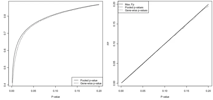
4.2.2 Gene-wise p-values Versus Pooled p-values ... 47

4.2.3 Proposed Moderation for Different Quantiles ... 50

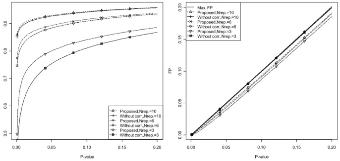
4.2.4 The Proposed VSP Method using Different Number of Replicates ... 51

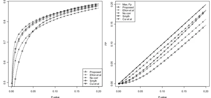
4.2.5 Performance Comparison of the Proposed Method with Existing Moderation Techniques ... 52

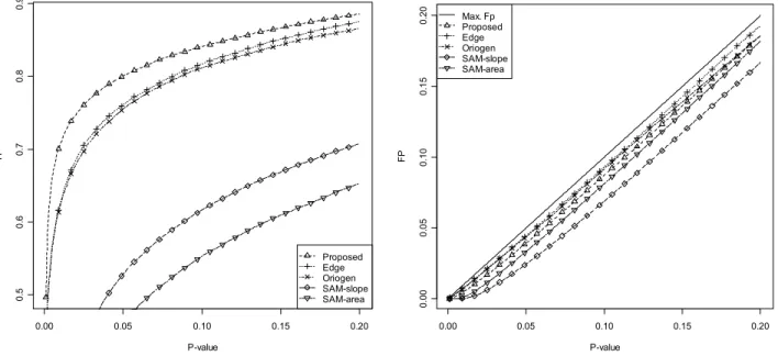
4.2.6 Performance Comparison of the Proposed Method with Existing Time-series Methods ... 54

viii

4.3 Results for Multiple Time-course Data ... 64

4.3.1 Performance Comparison of the Proposed Method with Existing Moderation Techniques ... 64

4.3.2 Performance Comparison of the Proposed Method with the Existing Time-series Methods ... 65

4.3.3 Results Using Real Dataset ... 66

4.4 Summary ... 68

Reconstruction of Gene Regulatory Network ... 70

Chapter 5 5.1 Gene Dependency Networks ... 70

5.1.1 Partial Correlation ... 71

5.1.2 The Graphical Model for Gene Dependency Networks ... 72

5.2 Gene Regulatory Network Model ... 72

5.2.1 The Graphical Model ... 74

5.2.2 Time Delay Estimation ... 74

5.2.3 Model Structure and Parameter Reconstruction ... 78

5.2.4 Adaptive Lasso ... 84

5.3 Summary of the Proposed Approach DD-lasso ... 85

Experimental Results on Network Reconstruction ... 87

Chapter 6 6.1 Synthetic and Real Datasets Description ... 87

6.2 Partial Correlation Dependency Networks ... 89

6.3 Network Reconstruction Results Using Synthetic data ... 90

6.3.1 The Performance of the Delay Detection ... 91

6.3.2 The Performance of the Lasso Regularization Parameter Selection ... 92

6.3.3 The Performance of the Proposed Delay Detection-lasso (DD-lasso) ... 98

6.3.4 The Effect of Backward-Elimination ... 100

ix

6.3.6 The Performance of the Proposed Adaptive DD-lasso and Adaptive Lasso ... 104

6.3.7 Comparison of the Proposed Approach with Existing GRN Reconstruction Methods ... 106

6.4 Results of Network Reconstruction Using Real data ... 109

6.4.1 Dataset 1 ... 109 6.4.2 Dataset 2 ... 111 6.5 Summary ... 114 Conclusion ... 115 Chapter 7 7.1 Concluding remarks ... 115

7.2 Scope for further investigation ... 118

References ... 119

x

List of Figures

Figure 1.1 Two-channel Microarray formation process ... 3

Figure 1.2 Output Microarray image ... 4

Figure 2.1 Network architectures ... 17

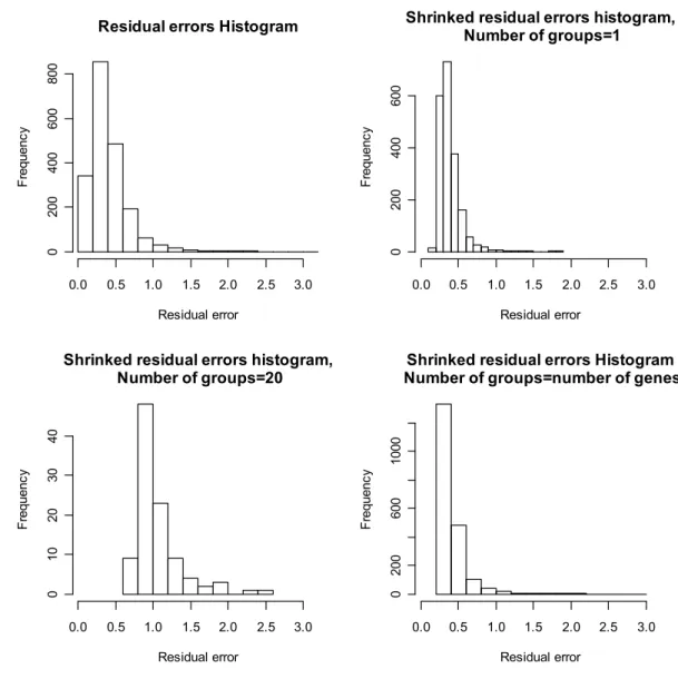
Figure 3.1 The shrinkage parameter for different number of groups. ... 30

Figure 3.2 Histograms of the residual errors for different number of groups. ... 31

Figure 4.1 Examples of the generated time series, si(t). ... 42

Figure 4.2 Examples of the generated time series, ri(t). ... 44

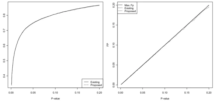
Figure 4.3 TP and FP for the existing and proposed gene-wise p-values methods. ... 47

Figure 4.4 TP and FP for the gene-wise and pooled p-values methods. ... 48

Figure 4.5 TP and FP for the gene-wise and pooled p-values methods in the heterogeneous case. ... 49

Figure 4.6 TP and FP for the proposed moderation technique. ... 50

Figure 4.7 TP and FP for the proposed moderation for different number of replicates. ... 52

Figure 4.8 TP and FP for the different moderation techniques for the first error model. ... 53

Figure 4.9 TP and FP for the different moderation techniques for the second error model. ... 53

Figure 4.10 TP and FP for several time-series methods for the first error model (a). ... 55

Figure 4.11 TP and FP for several time-series methods for the second error model (a). ... 55

Figure 4.12 TP and FP for several time-series methods for the first error model (b). ... 56

Figure 4.13 TP and FP for several time-series methods for the second error model (b)... 57

Figure 4.14 (a) Upregulated genes. (b) Downregulated genes. ... 61

xi

Figure 4.16 Gene Expressions for 6 clusters ... 62

Figure 4.17 Scatter plot of residual errors for non-differeentially expressed genes ... 63

Figure 4.18 Scatter plot of residual errors for differeentially expressed genes ... 63

Figure 4.19 TP and FP for the different moderation techniques ... 65

Figure 4.20 TP and FP for several time-series methods ... 66

Figure 4.21 Genes expressions of the the two siginficant genes missed by other techniques .... 67

Figure 4.22 Gene Expressions of significant genes where cold stress are solid lines, while control are dashed lines. ... 68

Figure 5.1 Autocorrelation of a signal s(t) ... 75

Figure 5.2 Cross-correlation between the two signals s(t) and s(t-3) ... 76

Figure 6.1 TP rate, FP rate and F1-measure at T=10 and T=20 for cross-validation ... 93

Figure 6.2 TP rate, FP rate and F1-measure at T=10 and T=20 for BIC criterion ... 95

Figure 6.3 TP rate and FP rate for various α ... 96

Figure 6.4 Precision, P, and Recall. R, for various α ... 96

Figure 6.5 F1-measure for various ... 97

Figure 6.6 Bar plot of the average Precision and Recall of 300 networks for each n ... 99

Figure 6.7 Bar plot of the average Precision and Recall of 300 networks for each n ... 101

Figure 6.8 Precision and Recall for DD-lasso with backward elimination at different delays.103 Figure 6.9 Bar plot of the average Precision and Recall ... 107

Figure 6.10 Hela cell cycle network, where true edges are solid lines, while false edges are dashed lines ... 111

xii

xiii

List of Tables

Table 1-1 Microarray data for each gene ... 4

Table 3-1 Data arrangment for each gene ... 25

Table 3-2 Range of residual sum of squares ... 32

Table 3-3 Data arrangment for each gene. ... 38

Table 4-1 Sensitivity and Specificity for the Existing and Proposed gene-wise p-values methods ... 46

Table 4-2 Sensitivity and Specificity for the gene-wise and pooled p-values methods ... 49

Table 4-3 Sensitivity and Specificity for the gene-wise and pooled p-values methods ... 49

Table 4-4 Sensitivity and Specificity for the proposed moderation technique ... 51

Table 4-5 Sensitivity and Specificity for the proposed moderation technique ... 51

Table 4-6 Sensitivity and Specificity for the moderation methods ... 54

Table 4-7 Sensitivity and Specificity for the Time-series Methods (a)... 56

Table 4-8 Sensitivity and Specificity for the Time-series Methods (b) ... 57

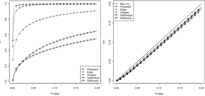
Table 4-9 Summary of the genes identified by the proposed VSP method and EDGE method . 59 Table 4-10 Sensitivity and Specificity for the moderation methods ... 64

Table 4-11 Sensitivity and Specificity for the Time-series Methods ... 65

Table 6-1 Partial corrlation results ... 90

Table 6-2 TP rate of delays for the three correlation methods ... 91

Table 6-3 Results for 10-fold cross validation ... 92

Table 6-4 Results for BIC criteria ... 94

xiv

Table 6-6 Results for the F1-measure of CV, BIC and mBIC2 criterion ... 98

Table 6-7 P, R and F1 for DD-lasso ... 100

Table 6-8 TP rate and FP rate for DD-lasso ... 100

Table 6-9 Results for the F1-measure of DD-lasso with and without backward elimination .. 101

Table 6-10 Results of P, R, TP rate and FP rate for DD-lasso with and without backward elimination ... 102

Table 6-11 Results of P, R and F1 for DD-lasso other delays ... 102

Table 6-12 TP rate and FP rate for DD-lasso with and without backward elimination ... 103

Table 6-13 F1 for Adaptive DD-lasso ... 104

Table 6-14 P, R, TP rate and FP rate for Adaptive DD-lasso ... 105

Table 6-15 P, R and F1 for Adaptive DD-lasso with backward elimination ... 105

Table 6-16 Results for the F1-measure of Proposed DD-lasso, Group lasso and Tlasso ... 108

Table 6-17 Results of P, R TP rate and FP rate for existing methods ... 108

Table 6-18 Computational time in seconds for the proposed and existing methods ... 109

Table 6-19 Results for the hela cell cycle ... 111

xv

List of Abbreviations

ANOVA Analysis of variance cDNA Complementary DNA DD-LASSO Delay Detection LASSO DNA Deoxyribonucleic acid EA Evolutionary algorithm EM Expectation-Maximization FDR False Discovery rate GRN Gene Regulatory Network LARS Least Angle Regression

LASSO Least Absolute Shrinkage and Selection Operator MOEA Multi-objective Evolutionary Algorithm

MOP Multi-objective Optimization Problem ODE Ordinary Differential Equation

PCA Principal Component Analysis RM ANOVA Repeated Measures ANOVA RNA Ribonucleic acid

SVD Singular Value Decomposition TF Transcription Factor

1

Chapter 1

Introduction

In DNA gene expression microarrays thousands of gene expression levels are measured simultaneously. Microarray data may provide insight into gene to gene interactions, gene function and pathway identification. Expression microarrays can be studied for static or temporal data. In a static experiment, the arrays are obtained at a single moment of gene expression. In a time series experiment the arrays are collected over a time course, allowing the study of the dynamic behavior of gene expression. Since the regulation of gene expression is a dynamic process, it is vital to identify and characterize changes in gene expression over time. In this work we are mainly interested in the time course data. The key challenges for the time series data are that the number of time points as well as the number of samples is small and the number of genes is very large.

The main microarray data analysis steps involves the identification of differentially expressed genes, gene clustering and gene regulatory network reconstruction. The identification of differentially expressed genes is to find genes whose expression changes in response to different biological conditions, which is a vital step of microarray data analysis. In this inference process, two essential steps are needed; the definition of the statistic measuring the differential expression, which enables us to rank the genes, and the assessment of the statistical significance of the results.

The aim of regulatory network reconstruction is to detect the most likely interactions by identifying sets of relevant model parameters that are required to obtain an appropriate correspondence between measured data and model output.

This work is concerned with the identification of differentially expressed genes and the network reconstruction. The gene selection is an essential primary step while the network inference gives more understanding of the underlying biological processes.

A microarray background and microarray data preprocessing background are found in the next two sections. Then, problem statement and research objectives are introduced in the following sections, followed by a brief description of the thesis organization in the last section.

2 1.1 Gene Expression Microarrays

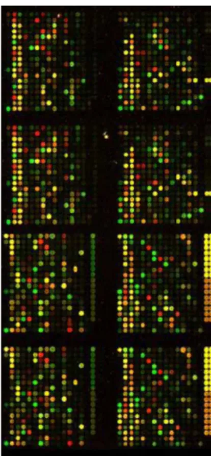
The main nucleic genetic material of cells is represented by Deoxyribonucleic acid (DNA) molecules. It is a nucleic acid that contains the genetic information for the development and functioning of all living organisms. The DNA double helix molecules comprise two anti-parallel intertwined complementary strands. The genetic information in a living organism is the same in all cells. Nevertheless, according to the different types of cells and responses only some genes would be active (expressed). Expressed genes show how the cells function and the underlying biological processes. A gene is expressed when it makes a new protein. Transcriptional gene regulation is a process where the DNA of a certain gene is used as a template. This gene is translated later to a protein. The better understanding of these gene transcription activities lead to accurate understanding of the underlying cellular processes and responses. In the transcription process, hybridization occurs, where part of the DNA binds with the mRNA. The microarray technology repeats the hybridization process to know which genes are expressed.

DNA microarrays are used to measure changes in expression levels. Microarrays differ in fabrication, workings, accuracy, efficiency, and cost. A microarray is usually a slide containing large number of tiny spots consisting of probe sequences. They can be immobilized at micrometer distances, so it is possible to place many different probes on a small single surface of one square centimeter. The number of probes can reach 10,000 or more. Target RNA is generally extracted from samples of interest (e.g. cancer tumors), reverse transcribed into complementary DNA (cDNA), labeled with fluorescent dye and then hybridized to the array. There are one channel and two channel microarrays. The more common arrays are the two color arrays, where two different samples are labeled with different dyes (Cy3, green and Cy5, red), and then, hybridized simultaneously to the same slide. Two DNA strands hybridize if they are complementary to each other. One or both strands of the DNA hybrid can be replaced by RNA and hybridization will still occur as long as there is complementarity. The fluorescent intensity of a spot is equivalent to the amount of RNA expressed in the sample. The fluorescent dye can be detected by a light scanner that scans the surface of the chip for hybridized material. A summary of the microarray process for a two channel microarray is shown in Figure 1.1. Hybridization both labeled samples are mixed

3

purified and hybridized on the microarray base pair interactions between DNA samples(target) and DNA molecules on the microarray (probes). Usually green spots indicate only DNA from probe is fixed, while red spots mean only DNA from the experimental sample is fixed, whereas yellow spots show that DNA from both are fixed in equal amount, and grey spots appear when there is no hybridization. A sample of microarray image is shown in Figure 1.2.

Figure 1.1 Two-channel Microarray formation process

In time series microarray data, the arrays are collected over a time course. Usually, microarray experiments are very noisy and there are lots of sources of error; hence, it is recommended to replicate the experiment several times to ensure the quality of the gene expression data. The microarray data measurements are repeated to form replicated samples. Then, the resulting microarray image is preprocessed, to get numerical values for each gene, known as gene expression data, and arranged in tables as shown in Table 1-1.

4

Figure 1.2 Output Microarray image Table 1-1 Microarray data for each gene

Time point 1 ……. Time point j ……. Time point T Sample 1 ….. Sample i Yij ….. Sample n

1.2 Preprocessing of Microarray Data

First, the raw microarray data is preprocessed in order to minimize extraneous variations in the measured gene expression levels of hybridized mRNA samples, and the biological variations can be

5

more easily distinguished. An essential step of data preprocessing is to normalize the microarray data, where normalization is the process of removing systematic variation from the data. Systematic errors in DNA microarray experiments can result from unequal RNA quantities in the sample, differences in labeling and detection efficiencies. In addition to that, errors can be due to systematic biases in measured expression levels, scanner settings, laser saturation effects, print-tip variation and sample plate origin. Normalization adjusts individual intensities so that comparisons can be made both within an array and between arrays in the experiment. Adjustments are necessary to remove differences which are purely technical and do not represent true biological variation. The purpose of normalization is to adjust for effects which arise from variation in the microarray technology rather than from biological differences between the RNA samples or between the printed probes. These differences if left unadjusted will hinder the ability to identify true differentially expressed genes (i.e. detect the genes that are actually active and producing proteins) and may increase the number of false positives found. In order to remove the bias artifacts, sophisticated methods have to be applied. If the imbalance is more complicated than a simple scaling of one channel relative to the other, as it usually will be, then the dye bias is a function of intensity and normalization will need to be intensity dependent. The dye-bias will also generally vary with spatial position on the slide. Positions on a slide may differ because of differences between the 2 print-tips on the array printer, variation over the course of the print-run, non-uniformity in the hybridization or from artifacts on the surface of the array which affect one color more than the other. Finally, differences between arrays may arise from differences in print quality, from differences in ambient conditions when the plates were processed or simply from changes in the scanner settings. There are many other trends which could be estimated and adjusted for in the normalization step, although normally these are of less importance than the intensity and spatial trends already considered. For example, there can be differences between the purity of DNA from different amplification batches or from different clone libraries. This can mean that different spots on the microarray contain different effective quantities of DNA. Normalization not only corrects for different dye properties but also for concentration differences between the co-hybridized test and reference samples. The locally weighted linear regression (LOWESS) normalization and the

6

quantile normalization are able to correct intensity-dependent effects. After the normalization and scaling steps, microarray analysis can be applied to extract meaningful information from this microarray data.

1.3 More Recent Technologies for Gene Expression Data

In this thesis, we carry out the analysis of time-series gene expressions that are extracted from microarray data, since currently hybridization-based microarrays are the primary method for global gene expression analysis and microarray databases are easily available. The same analysis methods and techniques can be safely applied to time-series gene expression data that is generated using more recent technologies such as more advanced probe-based methods (e.g. Nanostring) [1] and RNA sequencing (RNA-Seq) [2] methods.

The Nanostring technology [1] is a variation of the DNA microarray where it uses molecular barcodes and microscopic imaging to detect and count up to several hundred unique transcripts in one hybridization reaction. Each color-coded barcode is attached to a single target-specific probe corresponding to a gene of interest. This technology employs two ~ 50 base probes per mRNA that hybridize in solution. The Reporter Probe carries the signal; the Capture Probe allows the complex to be immobilized for data collection. After hybridization, the excess probes are removed and the probe/target complexes aligned and immobilized in the nCounter Cartridge. Sample Cartridges are placed in the Digital Analyzer for data collection. Color codes on the surface of the cartridge are counted and tabulated for each target molecule.

RNA-Seq [2] has the potential to replace microarrays in transcriptome analysis due to its advantages in sensitivity, quantification, and replicability of experiments. RNA-Seq allows the sequencing of the entire transcriptome, and thus permits both transcript discovery and robust digital quantitative analysis of gene expression levels. This method relies on the generation of short reads of transcript sequence information which are then assembled into full-length transcripts and mapped to the genome. To generate this data, isolated RNA populations (e.g. small RNAs) are converted to cDNA for sequencing More recently developed methods involve direct sequencing of RNA to avoid artifacts generated by reverse transcription and subsequent modification steps The number of reads

7

for a given transcript (calculated in reads per kilobase of exon model per million reads, or RPKM) corresponds to the absolute expression level of that particular gene in the cell type or tissue in question, providing an absolute quantification method with large dynamic ranges in contrast to the relatively limited dynamic range of microarrays that depends on relative, rather than absolute, quantification of hybridization intensities.

1.4 Motivation

The understanding of the gene interactions that contribute to certain diseases provides a potential therapeutic strategy. A comprehensive investigation of the microarray data is a possible way to get such a detailed understanding. Identifying which genes are differentially expressed in treated samples followed by modeling these differentially expressed genes provide deep insight into the biological interactions and processes.

There are a limited number of methods that have been proposed for selecting the genes that exhibit changes with time. There are four main approaches that have been proposed to solve this problem. Peddada et al. [3] have identified genes by comparing each of the gene expressions with predefined candidate profiles. Hence, the larger the number of time points, the larger the set of predefined profiles that need to be used. Storey et al. [4] have determined significant genes by performing on each gene a hypothesis test to determine as to whether its population-average versus time curve is flat. Hence, any significant change at a single time point is missed, and only significant change at continuous time changes can be identified. Tai et al. [5] have used an empirical Bayes method to identify highly-expressed genes. However, this method does not provide explicit p-values or q-values for the genes, but it only ranks the genes according to their significance. Angelini et al. [6] have proposed a Bayesian approach in which each gene expression profile is estimated globally by expanding it over an orthogonal basis. Nevertheless, some model parameters need to be defined such as the degree of the polynomial and the maximal possible degree. The existing methods for identifying significant genes changing with time, still needs accurate study and improvements. Hence, there is a need to identify significant genes while avoiding previous drawbacks, such as setting prior model parameters, to identify significant genes

8 irrespective of the type of change with time.

Dependency networks such as that in [7-9] that are based solely on correlations have several shortcomings. The resulting networks are undirected graphs that do not provide sufficient information regarding the relationships between the various genes. In addition, whenever any two genes are correlated to a third gene, the first two genes will be falsely connected, thus resulting in triangular clusters of genes that do not represent the real topology of GRNs. This is a major drawback of such dependency networks. Further, such networks do not take into consideration the delays between various genes, which is an inherent property of GRNs. Since GRN is an abstract network, where there is underlying chemical reactions and biological processes, time delays between stimulus and response exist that should not be neglected. In fact, physical interactions between genes are mediated through other components such as DNA, RNA, proteins, and metabolites, and gene networks are system-level descriptions of cellular physiology. Hence, incorporating delays in the GRN model is an essential part for successful modeling. An approach for GRN reconstruction that takes into account the time delays is one where the delays are represented by a system of equations, such as in [10-15].

The previous works in [7-9] consider the relations between genes without any delay. On the other hand, approaches such as in [10, 11, 15] incorporate a fixed time delay in their model. Li et al.[12] have developed a GRN with variable time delays. They use a decision tree to discover the time-delayed regulations between the underlying genes. Hence, they need additional datasets for training before they can apply their method successfully. Lozano et al.[13] have used a group lasso penalty in order to obtain a Granger graphical model. The group lasso penalty considers all the different time lags and indicates X to be Granger-causal for Y, if it has a significant effect. Since the average effect of all time lags is studied as one feature, the actual time difference between the activation of X and its effect on Y is still unknown. In addition, due to the averaging effect, it is not possible to determine the actual effect of X on Y, as to whether it is positive or negative. Shojaie et al.[14] have proposed a truncating lasso penalty for the estimation of graphical Granger models. The truncating effect of the proposed penalty is motivated by the rationale that the number of effects (edges) in the graphical model decreases as the time lag increases. Consequently, if the number of

9

edges is less than a predefined number at time t, all the later estimates are forced to be zero. They apply a stopping condition to stop adding more delays in the model to provide an estimate of the order of the underlying model. However, in order to do so, they require a large number of samples, and in addition, they completely ignore all the samples of further time points.

A major drawback of all the above mentioned approaches is that they are not able to model the variable time lags between any two genes, without the need for a large number of data sets or samples. When a gene regulates another gene, there is a delay before the response of the second gene appears. This delay is attributed to the underlying biological processes, such as transcription and translation that are taking place. The main challenge in modeling such time delays arises from the fact that the amount of delay is unknown between the various genes.

1.5 Objectives of the thesis

The overall objective of this study is to have a better understanding of the various biological processes using microarray data. This is achieved by addressing the following two key problems. What are the genes whose gene expressions change with time? How do these genes interact? Answers to these questions are attempted in two parts. First, new techniques are developed to infer the differential gene expressions over time. The main challenge in this part is the large number of genes whereas the number of samples is small. Second, gene regulatory network model need to be reconstructed from the gens selected from the first part. Successful gene reconstruction will yield a dynamic model that would describe the biological interactions and dynamics for various conditions. The key limiting factor is the very limited number of time points and samples compared to the number of genes composing the network. Since the number of model parameters is large compared to the available measurement data, the system is usually underdetermined. In general, without constraints, there are multiple solutions and the system of equations is not uniquely identifiable from the microarray data. It is required to obtain an appropriate system despite the non-identifiable parameter values. Thus, the identification of model structure and model parameters requires constraints representing prior knowledge, simplifications or approximations. Expression level of genes in a given cell can be influenced by a pathological status, a pharmacological or medical

10

treatment. The response to a given stimulus is usually different for different genes and depends on time.

Thus, the main objectives of the present work are to detect differential gene expressions over time, and to infer a detailed GRN structure, using time-series microarray data, that detects the most likely gene interactions taking into account the possible delays between different genes and to distinguish between the direct and indirect relationships. Successful gene reconstruction will provide valuable information for the pharmaceutical and biotechnology industries to design new drugs for complex diseases.

1.6 Thesis Organization

The organization of the thesis is as follows. An overview of the statistical background and the current literature for the identification of differentially expressed genes, and the gene regulatory network reconstruction are provided in Chapter 2. In Chapter 3, a detailed description of the proposed methodologies for the identification of differentially expressed genes is presented. Experimental results concerning the performance of the proposed methodologies for the identification of differentially expressed genes are given in Chapter 4. Then, the proposed approach for network reconstruction is described in Chapter 5. The experimental results concerning the performance of the approach for network reconstruction are illustrated in Chapter 6. The conclusions are summarized in Chapter 7. Finally, the R code of the proposed methods are found in the appendix.

11

Chapter 2

Literature Review

First, statistical background is introduced in the first section, followed by the previous work for the identification of the differentially expressed genes and the network reconstruction are found in the following two sections. Then, a brief summary is presented in the last section.

2.1 Statistical Background

2.1.1 Hypothesis Testing

In order to identify differentially expressed genes, hypothesis testing is applied. In a hypothesis test, there is an initial research hypothesis of which the truth is unknown. Then, the first step is to state the relevant null, H0, and alternative hypotheses. Afterwards, decide which test is appropriate,

and state the relevant test statistic. Subsequently, the distribution of the test statistic under the null hypothesis is either derived from the assumptions, or the test statistic follows a standard distribution, such as the Student's t distribution or normal distribution. Then, from the observations the observed value tobs of the test statistic T is computed. Select a significance level (α), a

probability threshold below which the null hypothesis will be rejected, while common values of α

are 5% and 1%. According to the distribution of the test statistic under the null hypothesis, a probability of the observation under the null hypothesis (the p-value) is calculated. The decision rule is to reject the null hypothesis if and only if the p-value is less than the significance level (the selected probability) threshold.

P-value is a measure of the evidence against the null hypothesis in a statistical test. It is the probability of the occurrence of a test statistic equal to, or more extreme than, the observed value under the assumption that the null hypothesis is true. As in any other statistical test, the decision is made by comparing the reference value of the test statistic (t) to the reference distribution obtained under H0. If the reference value of t is typical of the values obtained under the null hypothesis, H0

cannot be rejected; if it is unusual, being too extreme to be considered a likely result under H0, H0 is

12

distribution of the test statistic under the null hypothesis can be derived using resampling techniques.

2.1.2 Resampling Techniques

Resampling is a nonparametric method of statistical inference, that does not involve the utilization of the standard distribution tables (for example, normal distribution tables) in order to compute approximate probability values. It is used as a robust alternative to inference based on parametric assumptions when those assumptions are in doubt, or where parametric inference is impossible or requires very complicated formulas for the calculation of standard errors. These techniques include the bootstrapping as well as the permutation significance tests.

Bootstrapping is a statistical method for estimating the sampling distribution of an estimator by sampling with replacement from the original sample in such a manner that each number of the sample drawn has a number of cases that are similar to the original data sample. Due to replacement, the drawn number of samples that are used by the method of Resampling consists of repetitive cases. It can be used for constructing hypothesis tests. A permutation test is a statistical significance test in which a reference distribution is obtained by calculating all possible values of the test statistic under rearrangements of the samples. If the samples are exchangeable under the null hypothesis, then the resulting tests yield exact significance levels. Confidence intervals can then be derived from these tests. The leading assumption is that it is possible that all of the treatment groups are equivalent, and that every member of them is the same before sampling began. From this, one can calculate a statistic and then see to what extent this statistic is special by seeing how likely it would be if the treatment assignments had been rearranged.Permutation tests exist for any test statistic, regardless of whether or not its distribution is known. The argument invoked to construct a null distribution for the statistic is that, if the null hypothesis is true, all possible pairings of the two variables are equally likely to occur. The pairing found in the observed data is just one of the possible, equally likely pairings, so that the value of the test statistic for the unpermuted data should be typical, i.e. located in the central part of the permutation distribution.

13

with sampling with replacement while for permutation test the sampling is done without replacement. Moreover, Permutations test hypotheses is concerned with the distributions while bootstraps test hypotheses is concerned with the parameters.

2.2 Identification of Differentially Expressed Genes Literature Review

Early work for identifying differentially expressed gens was done by using a fixed threshold value, such as using a two-fold increase. However, this is statistically inadequate. There are large number of random biological variations that can occur during a microarray experiment, such as sample-to-sample differences and physiological variations. A more appropriate approach for the identification of differentially expressed genes includes calculation of a statistic based on replicate array data for ranking genes according to their possibilities of differential expression and selection of a cut-off value for rejecting the null-hypothesis that the gene is not differentially expressed.

2.2.1 Time Series Identification of Differentially Expressed Genes Review

Some of the previous work was originally done for static gene expressions (i.e. gene expressions are measured at a single time point) such as that of Tusher et al. [16] and was subsequently extended to time-course expressions in SAM (http://www-stat.stanford.edu/~tibs/SAM). However, since the main research work was carried out on static data there is no statistical validation for the genes identified. Some of the other research groups have focused on identifying differential genes for time series expressions among different classes. For instance, Park et al. [17] have proposed a statistical test procedure based on the ANOVA model where the effect of time is first removed and then the residuals are used.

There are a limited number of methods that have been proposed for selecting the genes that exhibit changes with time. There are four main approaches that have been proposed to solve this problem.

Peddada et al. [3] have identified genes by comparing each of the gene expressions with predefined candidate profiles. The candidate profiles are expressed in terms of the inequalities between the expected expression levels at different time points. Hence, the larger the number of

14

time points, the larger the set of predefined profiles that need to be used. The best fitting profile for a given gene is selected based on the goodness-of-fit criterion and the bootstrap test. A bootstrap test procedure is conducted for each gene independent of the other genes. This algorithm could be useful for classification purposes. If the differential genes are already known, this test can be used to easily identify different profiles. Storey et al. [4] have determined significant genes by performing on each gene a hypothesis test to determine as to whether its population-average versus time curve is flat. A statistic analogous to the t and F statistics has been defined. Two models, one based on the approximation of the population-average versus time curve by a polynomial and the other by a natural cubic spline have been proposed. The model fitting procedure for longitudinal sampling is much more complicated since it takes into account the dependency of the measurements for a given subject. A false discovery rate criterion is then applied and the q-values for the genes estimated. Any significant change at a single time point is missed, and only significant change at continuous time changes can be identified.

Tai et al. [5] haveused an empirical Bayes method to identify highly-expressed genes.They have derived the corresponding statistics for both the one-sample and two-sample problems, where in the former, the null hypothesis is that the expected temporal profile is constant, while that in the latter, the two expected temporal profiles are the same. However, this method does not provide explicit p-values or q-p-values for the genes, but it only ranks the genes according to their significance.

Angelini et al. [6] have proposed a Bayesian approach in which each gene expression profile is estimated globally by expanding it over an orthogonal basis. Each gene expression profile is presented by a short vector of coefficients and Bayesian approach delivers the posterior distribution of this vector. The method can accommodate various types of error distributions such as the normal, Student T and double-exponential. Since all the computations are performed analytically, the application of resampling methods is avoided. Nevertheless, some model parameters need to be defined such as the degree of the polynomial and the maximal possible degree. Their model can be useful for generating simulation data and is available in their software BATS [18].

15

differential expression namely, the statistic, and the assessment of the statistical significance of the results. In the microarray data, due to the small number of samples, the statistic may need moderation. Moderation is well-studied in the microarray literature as shown in the next subsection.

2.2.2 Variance Moderation Review

Baldi and Long [19] have implemented an empirical Bayes approach, where population variances were estimated by a weighted mixture of the sample variance and an overall factor selected using expression values from all the data. The moderated t-test replaces the usual variance estimate with a Bayesian estimator based on a hierarchical prior distribution. Efron et al. [20] have added a factor to the denominator of the statistic. This additional factor is the same for all the genes and is commonly chosen from the set of pooled standard deviations. They have chosen the factor as a quantile of the standard deviation values of all the genes. Tusher et al. [16] have implemented a procedure to choose the factor automatically. They have estimated the factor among the percentiles of the standard errors by minimizing a coefficient of variation. The coefficient of variation of the median absolute deviation of the test statistic is computed over a number of percentiles. Broberg [21] has proposed a computationally intensive method to determine the added factor by minimizing a combination of estimated false positive and false negative rates over a grid of significance levels and factors. Smyth [22] has used an empirical Bayesian technique, where small variances are raised and large variances shrunken towards a common value. Cui et al. [23] have proposed a shrinkage estimator for gene-specific variance components based on the James–Stein estimator and have used it to construct a test statistic. The shrinkage estimator makes a priori assumptions about the distribution of the variance components. Wright et al. [24] have proposed a model, where the within gene variances are drawn from an inverse gamma distribution, whose parameters are estimated across all genes. Most of the proposed correction algorithms are defined and applied for the t-test only. Smyth [22], Cui [23] and Wright et al. [24] have proposed extensions to their algorithm to the multi-groups testing and the F test. Nonetheless, they have distribution assumptions for the residual error.

16

either the permutations of the whole set of genes (pooled) [4, 25] or the permutations of each gene independently (gene-wise) [3, 17, 26].

After identifying the significant genes, the next step is to understand the interactions between these genes through network reconstruction.

2.3 Network Reconstruction Literature Review

The observed changes in gene expression over time are either due to direct effects of the stimulus on specific genes or result from secondary gene to gene interactions. Genes are working in a cascade of networks; hence, there is growing interest in the use of expression data to construct biological networks. GRNs provide an understanding of the genetic architecture of complex diseases, and thus, assist in developing new therapeutic solutions. The goal of network inference is to detect the most likely interactions by identifying sets of relevant model parameters. Intensity values of samples are usually averaged to reduce the complexity of the data set. There are different network model architectures that can be employed to reconstruct the gene regulatory network (GRN). The model architecture is a parameterized mathematical function that describes the general behavior of a target component based on the activity of regulatory components. Once the model architecture has been defined, the network structure (i.e. the interactions between the components) and the model parameters (e.g. type/strengths of these interactions) need to be learned from the data. Over the last years, a number of different model architectures from gene expression data have been proposed. In general, the network nodes represent compounds of interest, e.g. genes or modules (sets of compounds). Model architectures can be distinguished by the representation of the activity level of the network components. Since both network structure and parameters are unknown, statistical approaches such as graphical models and linear systems are used to estimate the genetic networks. The concentration or activity of a compound can be represented by Boolean or other logic values, discrete, fuzzy or continuous values. Furthermore, network model architectures can be distinguished by the type of model (stochastic or deterministic, static or dynamic) and the type of relationships between the variables (directed or undirected; linear or non-linear function or relation table). The major network classes are the system of equations, Boolean

17

network, Bayesian network and the information theory architectures. The different network architectures are shown in Figure 2.1.

Figure 2.1 Network architectures

A drawback of the information theory models is that they are static, while that of the Boolean networks is that the gene expressions cannot be described adequately by only two states. The two models that best describe the dynamics are that the system of equation models and the Bayesian networks. The system of equations model has different aspects. The system of equation can be continuous (differential equations) or discrete (difference equations). Furthermore, the equations could be representing linear system or non-linear one. In addition to that, the system can be deterministic or stochastic taking into account the random variability of the gene expressions.

2.3.1 Information Theory Models and Measures of Association

If the network structure is unknown, statistical approaches such as graphical models are used to estimate genetic networks. It is mainly concerned with constructing Dependency Graphs between different genes. These graphs should reveal the distinction between direct and indirect interactions of various genes, thereby inferring the underlying network topology. Correlations are widely used to infer the structure of the GRN. In this regard, Opgen-rhein et al. [7] have used a functional approach to find the dynamic correlations between various genes. They have considered the

18

observed gene expressions over time as realizations of random curves, rather than considering the individual time points separately. They have approximated the temporal expression of the genes using linear splines. Their approach has been based on a dynamic pair-wise correlation estimator which provides a similarity score for pairs of groups of randomly sampled curves. They compute the partial dynamic correlations matrix directly from the inverse of the correlation matrix. De la Fuente et al. [8] have proposed a method to construct approximate dependency graphs from large-scale biochemical data using partial correlation coefficients. The partial correlations of first and second order are computed using iterative methods. The correlation between two variables is evaluated by conditioning on all possible pairs of other variables. If any of these pairs yields a zero partial correlation the corresponding edge is removed from the correlation network. This is executed over all possible edges results in a network of direct interactions. The conditioning on any common causal descendent introduces a correlation between two variables that are independent conditional on their causal ancestors. Therefore, conditioning on all variables simultaneously can introduce some dependencies, which are not due to direct causal effects or common ancestors. Wille et al. [9] have used only the first order partial correlations, where they have applied graphical modeling to sub-networks of three genes to study the dependence between two genes conditional on the third one. Then, the sub-networks have been combined for the inference of the complete network. Dependency networks that are based solely on correlations have several shortcomings. The resulting networks are undirected graphs that do not provide sufficient information regarding the relationships between the various genes. In addition, whenever any two genes are correlated to a third gene, the first two genes will be falsely connected, thus, resulting in triangular clusters of genes that do not represent the real topology of GRNs. This is a major drawback of such dependency networks. Further, such networks do not take into consideration the delays between various genes, which is an inherent property of GRNs. Since GRN is an abstract network, where there is underlying chemical reactions and biological processes, time delays between stimulus and response exist and should not be neglected. In fact, physical interactions between genes are mediated through other components such as DNA, RNA, proteins, and metabolites, and gene networks are system-level descriptions of cellular physiology. Hence, incorporating delays in the

19

GRN model is an essential part for successful modeling. An approach for GRN reconstruction that takes into account the time delays is one where the delays are represented by a system of equations.

2.3.2 System of Equations

There are two main approaches for modeling the network with linear System of Equations. One approach depends on reducing the problem of dimensionality while the other uses the global set of genes directly. In the first approach, the problem of large number of genes can be reduced first by applying gene clustering. The network is reconstructed between clusters, not each gene. Cluster-representative genes are used for the modeling. It could be assumed that genes which have similar expression patterns also have the same regulators. Another way for solving the underdetermined problem is to reduce the dimensionality of data using techniques such as the Principal Component Analysis (PCA) or the Singular Value Decomposition (SVD).

For instance, Guthke et al. [11] have used gene clustering combined with a heuristic search strategy for finding optimized network reconstruction. A modified fuzzy C-means algorithm has been employed for clustering. Afterwards, the network reconstruction has been composed of two parts the model structure and the model parameters. Prior knowledge concerning the connectivity between genes has been exploited to restrict the search space for the model structures.The model structure has been decomposed into smaller sub-models. The sub-model estimation starts with an initial sub-model that represents a first order lag element. The sub-model of each gene possesses two non-zero parameters; the parameter that realizes the self-regulation effect and the parameter that describes the influence of the external stimulus on the expression of the gene.Two directions of search have been applied; forward selection and backward elimination. For each model structure the model parameters have been fitted to the gene expression data using standard optimization techniques. Then, the mean square error between the model output and the data has been determined and used to assess the model structure. In order to find initial parameter values for the iterative optimization procedure, time derivatives have been used. They are calculated based on an interpolation between the data points. A drawback of the interaction networks between nodes of representative gene clusters is that the resulting network is an abstract network between gene

20

clusters. On the other hand, the gene regulatory networks of single genes give more insight into the various biological processes.

Bansal et al. [10] have inferred the local network of gene to gene interactions surrounding a gene, or genes, of interest by perturbing only one of the genes in the network and measuring the gene expression profiles at multiple time points. To solve the underdetermined system problem several steps have been applied. First, they have applied a cubic smoothing spline filter with an adjustable smoothing parameter. The purpose of the smoothing is to reduce the noise. Afterwards, they have used interpolation to increase the number of time points using piecewise cubic spline interpolation. Finally, PCA has been applied to the dataset in order to reduce its dimensionality and solve the equation in the reduced dimension space. It works on small size networks. Nonetheless, for very large number of genes its performance deteriorates.

Holter et al. [27] have used Singular value decomposition (SVD) to solve the linear equation system. The time evolution of gene expression levels has been described by using a time translational matrix to predict future expression levels of genes based on their expression levels at some initial time. The time translational matrix has been deduced by modeling them by using the characteristic modes obtained by singular value decomposition. The expression data for each gene is viewed as a unit vector in a hyperspace, each of whose axes represents the expression level at a measurement time of the experiment. The SVD construction ensures that the modes correspond to linearly independent basis vectors. A linear combination of these modes describes the expression pattern of each gene. The resulting time translation matrix has provided a measure of the relationships among the modes and governs their time evolution. They have showed that a truncated matrix linking just a few modes is a good approximation of the full time translation matrix. To solve the inverse problem and infer the nature of the gene network connectivity, the causal relationships among the characteristic modes obtained by SVD have been considered.

The second approach is to reverse-engineer the global genetic pathways without using data reduction techniques. Van Someren et al. [15] have developed an algorithm which is based on the Least Absolute Shrinkage and Selection Operator (lasso) technique. They have utilized the literature

21

enrichment scores to find parameter concerning the lasso technique. This enabled them to select a single network solution. Lasso [28] is an algorithm that shrinks the least absolute weights such that only a few weights remain non-zero. The linear model assumes that the gene expression level of each gene is the result of a weighted sum of all other gene expression levels at the previous time point. In order to obtain an estimate of the complete set of model parameters from data, usually the squared error between the predicted and measured gene expression levels is minimized. In lasso technique, the standard squared error with a penalty term that sums the absolute values of the weights is obtained. A parameter is multiplied by the penalty term. It provides a trade-off between data-fit term and the penalty term. The mathematical details of lasso and its implementation can be found in [28, 29].The properties and performance of lasso have been studied extensively and some improvements have been introduced. One of the most commonly-used modifications is that due to Zou [30]. He proposed an adaptive lasso penalty term which is weighted according to initial estimates and he has shown that if suitable weights are used, the adaptive lasso can achieve variable selection consistency.

All the previous work of [7], [8], and [9] consider the relations between genes without any delay. On the other hand, previous approaches, such as [10], [11]and [15], incorporate time delay in their model, however, they assume that all the genes are affected by other genes with a fixed delay. Li et al. [12] have developed a GRN with variable time delays. They have used a decision tree to discover the time-delayed regulations between the underlying genes. Hence, they need additional datasets for training before applying their method successfully to the problem of interest. Lozano et al. [13] have used a group lasso penalty in order to obtain a Granger graphical model. The group lasso penalty considers all the different time lags and indicates X to be Granger-causal for Y if the average effect is significant. Since the average effect of all time lags is studied as one feature, the actual time difference between activation of X and its effect on Y is still unknown. In addition, due to the averaging effect, it is not possible to determine the actual effect of X on Y as to whether it is positive or negative. Shojaie et al.[14] have proposed a truncating lasso penalty for the estimation of graphical Granger models. The truncating effect of the proposed penalty is motivated by the rationale that the number of effects (edges) in the graphical model decreases as the time lag

22

increases. Consequently, if there are less than a predefined number of edges at time at t, all the later estimates are forced to zero. They apply a stopping condition upon which they stop adding more delays in the model to provide an estimate of the order of the underlying model. However, in order to do so, they require a large number of samples, and in addition, they completely ignore all the samples of further time points.

2.4 Summary

As can be seen from the above literature review, the knowledge and understanding of the biological pathways are far from being complete. Clearly, a comprehensive investigation of the microarray data is a possible way to get detailed understanding. Identifying which genes are differentially expressed in treated samples is the first step to improve the biological understanding. As shown from the first section of the literature review, the existing methods for identifying significant genes changing with time, still needs accurate study and improvements.

The identified genes are used to reconstruct gene regulatory network for further understanding of the underlying dynamic processes. The GRN reconstruction is one of the major challenges in systems biology. A review of relevant literature studies demonstrates that the existing algorithms are of limited accuracy. A main drawback of all the previous approaches is that they are not able to model the variable time lags between any two genes, without the need for a huge number of data sets or samples. When a gene regulates another gene, there is a delay before the response of the second gene appears. This delay is attributed to the underlying biological processes taking place such as transcription and translation. The main challenge in these time delays is that the amount of delay is unknown between the various genes. There is a necessity to develop new techniques in these relatively new areas where studies devoted to these topics remain insufficient.

23

Chapter 3

Identification of Differentially Expressed Genes

In this work we are interested in the time-series data analysis. The first question as to which genes change their expressions is solved by identifying the differentially expressed genes [31]. For the first part, RM ANOVA will be used to get the statistic. Permutations are applied to get the p-values, and hence, determine the significance of the statistic. A new moderated statistic is introduced. For multiple time course data, a mixed design ANOVA is employed to compute the statistic, followed by a procedure similar to that of single time series.

3.1 Identifying Differentially Expressed Genes for a Single Time-course Data

In this section, an algorithm applicable to longitudinal time-series with samples is proposed for selecting genes according to their time-course profiles using gene expression data. The statistical inference consists of two main parts; definition of the quantity measuring differential expression, and assessing statistical significance of the results. In the proposed algorithm RM ANOVA will be used to get the statistic. To find its significance, permutations [32] are used to get the p-values. The methods of both the pooled p-values and the gene-wise p-values are used to evaluate the RM F significance. For the gene-wise p-values a new coarse-to-fine strategy is introduced to reduce the number of the required permutations. A new moderation factor is introduced and applied to the RM F-statistic.

3.1.1 RM ANOVA

Generally, ANOVA tests the null hypothesis of no differences between population means. One of the assumptions of ANOVA is the independence of the groups being compared. This is not true for longitudinal time-series data. Using a standard ANOVA in this case is not appropriate since it fails to model the correlation between the repeated measures. RM ANOVA takes into account these dependencies. The difference between the RM and the independent-measures (IM) ANOVA is that the former removes the variance caused by individual differences. Hypotheses for both the IM ANOVA and RM ANOVA are the same and test for the equality of the means. The mathematical

24 details of RM ANOVA can be found in [33].

The RM ANOVA may be thought of as a model designed to assess treatment differences while controlling the between-sample variability, when each gene expression value is measured a few consecutive times. The model is simple to interpret and takes into account the various aspects of the repeated-measurements data. The RM ANOVA model for each gene is given by [33]

Yij= η+μj+αi+ (αμ)ij +εij (3-1)

where Yij is the microarray value for the ith sample at the jth time point, η is the population grand mean under all fixed ratios, μj is the fixed effect of the time j, αi is the effect of the ith sample, αμij is the interaction effect and εij is the random error of the ith sample at the jth time point. The RM ANOVA model is similar to that of the mixed-effect where the replicated samples are the random variables and the time points are the fixed effect variable. The sample effects, αi’s, are assumed to be independent of one another and the errors, εij’s, are assumed to be independent of the other effects and of each other. The interaction term (αμ)ij of each sample is assumed to be independent of the interaction terms of the other samples, but can be dependent for the same subject. The null hypothesis, H0,states that the effect of time is constant across all time points, while the alternative

hypothesis, H1, states that there is a change across time. The hypothesis can be summarized as

follows:

H0: μ1 = μ2 = μ3 = …= μT

H1: H0 is false

In addition to the previous assumptions, in order to use the F-tables directly, it is assumed that the effect terms, the error term and the interaction term are normally distributed and that the variances of the differences for all time point combinations are homogeneous, which is known as sphericity. However, the normality assumption is not usually satisfied in the microarray data, and hence, instead of using the F-tables, permutation procedure is employed. In the null case, the correlation attributed to any changes with respect to time does not exist. Consequently, in addition to the mean, the variances and the pair-wise correlations between different measurements, for the same subject,

25

in the null case, are equal. This interpretation for the null case is sufficient for the validity of the application of the permutation procedure which is previously applied in [3, 17].

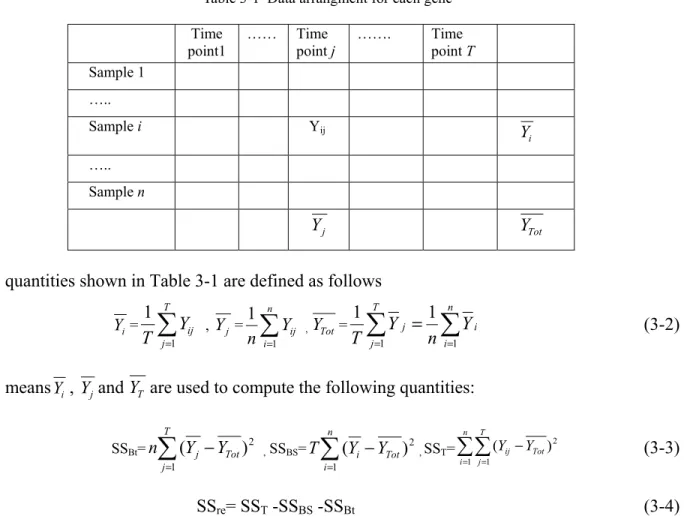
For each gene, data is arranged in a table with T-columns and n rows as shown in Table 3-1. The columns indicate the time points and rows the replicated samples. In this table, Yij is the microarray

value for the ith sample at the jth time point.

Table 3-1 Data arrangment for each gene Time

point1 …… Time point j ……. Time point T

Sample 1 ….. Sample i Yij i Y ….. Sample n j Y Y_Tot

The quantities shown in Table 3-1 are defined as follows

Y_i=









The meansY_i, Y_jandY_T are used to compute the following quantities:

SSBt=







where SSBt is the sum of squares of the treatment levels, SSBS is the sum of squares of the subjects,

SST is the total sum of squares and SSre is the residual (error) sum of squares, which is a measure of

the total discrepancy between a model and the observed data. These quantities are used to calculate the RM F-statistic using

26 F= re Bt SS SS n 1) ( − ( 3-5)

After computing the RM F-statistic, it is required to estimate the significance of these values for which the standard F-tables are generally used. Nonetheless, there are several assumptions required to use these F-tables. The main assumptions are that the observations among the individuals should be independent and should have normal distribution and variance homogeneity (sphericity). In case the sphericity assumption is violated, there are several methods to adjust the numbers of degrees of freedom, for example that of Geisser and Greenhouse [34]. However, in the present work the main assumption of normal distribution cannot be verified, and hence, the permutation based p-values are computed and used in the determination of the significance rather than using the standard F-tables. The permutation procedure is a valid approach for the time-series microarray data, where the null hypothesis tests if there is no effect of the time variable on any of the microarray data measurements, and that the measurements under the null hypothesis are assumed