R E S E A R C H
Open Access
Joint DOD/DOA estimation in MIMO radar
exploiting time-frequency signal representations
Yimin D Zhang
1*, Moeness G Amin
1and Braham Himed
2Abstract
In this article, we consider the joint estimation of direction-of-departure (DOD) and direction-of-arrival (DOA) information of maneuvering targets in a bistatic multiple-input multiple-output (MIMO) radar system that exploits spatial time-frequency distribution (STFD). STFD has been found useful in solving various array processing problems, such as direction finding and blind source separation, where nonstationary signals with time-varying spectral characteristics are encountered. The STFD approach to array processing has been primarily limited to conventional problems for passive radar platform that deals with signal arrivals, while its use in a MIMO radar configuration has received much less attention. This paper examines the use of STFD in MIMO radar systems with application to direction finding of moving targets with nonstationary signatures. Within this framework, we consider the use of joint transmit and receive apertures for the improved estimation of both target time-varying Doppler signatures and joint DOD/DOA. It is demonstrated that the STFD is an effective tool in MIMO radar processing when moving targets produce Doppler signatures that are highly localized in the time-frequency domain.
Keywords:radar signal processing, MIMO radar, direction finding, joint DOD/DOA estimation, time-frequency
ana-lysis, moving target tracking
1. Introduction
Multiple-input multiple-output (MIMO) radar is an emerging technology that has attracted significant inter-est in the radar community [1,2]. By emitting orthogonal waveforms from the transmit array antennas and utiliz-ing matched filterbanks in the receivers to extract the waveform components, MIMO radar systems can exploit the spatial diversity and the higher number of degrees of freedom to improve resolution, clutter miti-gation, and classification performance. In particular, a monostatic MIMO radar system exploiting colocated array antennas can provide effective array designs to achieve an extended virtual aperture which becomes the sum coarray of the transmit array and the receive arrays [2,3]. A bistatic MIMO radar with respectively colocated transmit and receive array antennas, on the other hand, is capable of jointly estimating the direction-of-depar-ture (DOD) and direction-of-arrival (DOA) of targets
[4-7]. There are various reasons motivating the use of bistatic radars, ranging from improving covertness to achieving improved location accuracy [8]. In the MIMO radar context, the combined DOD and DOA informa-tion allows triangulainforma-tion of target locainforma-tions. This is par-ticularly important in narrowband radar systems, such as over-the-horizon radar, which do not have a high range resolution [9]. The joint transmit and receive beamforming offers improved interference/jamming can-celation capability, which can be performed without the need for a priori information at the transmitter. This is made possible since the transmit beamforming is per-formed at the receiver [10].
Radar signals are often nonstationary with Doppler frequencies that may change slowly or rapidly with time. This is the case of Doppler signatures that are generated due to target move-ment and maneuvering. For those nonstationary signals, time-frequency distributions (TFDs) have been widely used as a powerful tool for sig-nal asig-nalysis, enhancement, and discrimination [11]. When used in array processing applications, time-fre-quency signal representations yield improved signature * Correspondence: [email protected]
1
Center for Advanced Communications, Villanova University, Villanova, PA 19085, USA
Full list of author information is available at the end of the article
detection, interference cancelation, direction estimation, and waveform recovery. In particular, the development of spatial time-frequency distribution (STFD) has led to a new paradigm for processing a large class of nonsta-tionary signals in multi-sensor array applications [12-24].
The STFD is defined by the STFD matrix, which includes the auto-sensor TFDs along its diagonal and cross-sensor TFDs as off-diagonal elements. The STFD matrix is related to the source TFD matrix by the spatial mixing matrix in a manner similar to the commonly used formula in array processing problems using sec-ond-order statistics that relates the sensor spatial covar-iance matrix to the source covarcovar-iance matrix. This similarity has enables eigenstructure and subspace meth-ods to play a role in high-resolution DOA estimation of nonstationary sources. It was shown in [19] that, by constructing an STFD matrix from the selected time-frequency points of highly localized signal energy, the corresponding signal and noise subspace estimates, as a result of signal-to-noise ratio (SNR) enhancement, become more robust to noise than their counterparts obtained using the data covariance matrix. In addition, the selected time-frequency points can pertain to a sin-gle or few sources, thus allowing the consideration of individual or subset of the sources in the field of view. The separability of the source time-frequency signature and the flexibility in time-frequency point set selection further increase the SNR and reduce the mutual inter-ference between the signals, yielding improved subspace robustness. Further, it allows processing more sources than the number of sensors. A number of direction find-ing techniques have been developed within the STFD framework to take advantages of the above properties (e. g., [13-15,17,20]). These techniques have shown improved performance compared to their conventional DOA approach counterparts.
The merits of time-frequency based DOA estimation can only be materialized through the selection of appro-priate time-frequency points in the construction of the STFD matrices. While in some scenarios the selection of peak time-frequency points may be relatively easy, the problem can be more challenging in other situations, e. g., when the signals are highly contaminated by noise. A typical radar return signal is very weak with a low SNR. Therefore, it becomes necessary to utilize the spatial diversity to enhance the time-frequency signature of the signals of interest in the absence of knowledge of their directions. A simple example for achieving this purpose is through averaging of the TFDs over all receive sen-sors [21]. The array averaged TFD also help in identify-ing auto-term and cross-terms points [22,23].
In this article, we consider the exploitation of STFD in bistatic MIMO radar applications. The goal is to
examine whether and how certain key advantages of the STFD, as described above, are preserved in the context of MIMO radar and their dependency on the number of transmit and receive antennas in bistatic MIMO sys-tems. In particular, we deal with two important issues. The first issue is the enhancement of auto-term TFDs in the presence of both cross-terms and noise to obtain reliable auto-term identification. The second issue is the joint DOD and DOA estimation within the time-fre-quency framework that allows target selection and dis-crimination through the proper selection of time-frequency regions. It becomes clear that cross-term reductions, due to the averaging operation of sensor TFDs, benefit from both transmit and receive array apertures, whereas the noise reduction is determined by the number of virtual antennas. It is shown that the joint DOD/DOA estimation performance is improved through time-frequency based target discrimination when a closely separated target is eliminated from the evaluation.
In the presence of multiple targets, a bistatic radar is required to properly pair the estimated DOD and DOA results. Several techniques have been developed to void or to automatically obtain pairing operation [5-7]. In this article, we develop our time-frequency domain DOD/DOA estimation technique based on the com-bined ESPRIT-MUSIC method [7], which only requires two decoupled one-dimensional direction finding opera-tions where the DOD and DOA are automatically paired.
The remainder of this article is organized as follows. The MIMO radar signal model is introduced in Section 2. The concept of STFD is reviewed in Section 3. The capability of enhancing the auto-term TFD over cross-term TFD and noise through averaging over virtual sen-sors is addressed in Section 4. Section 5 presents the joint DOD and DOA estimation in the time-frequency framework. Simulation results, validating our analyzes and discussion, are presented in Section 6.
The following notations are used in this article. A lower (upper) case bold letter denotes a vector (matrix). E[·] represents statistical mean operation. (·)*, (·)T, and (·)Hrespectively denote complex conjugation, transpose, and conjugate transpose (Hermitian) operations. Re(·) represents the real part operation of a complex variable,
vector or matrix.⊗denotes the Kronecker product and
◊denotes the Khatri-Rao product. Inexpresses then×
n identity matrix. Diag(x) denotes a diagonal matrix
using the elements of x as its diagonal elements, diag(X) a vector consisting of the diagonal elements of matrix
X, and vec(X) a vectorized result of matrix X. In
addi-tion, ℂN×M denotes the complete set ofN ×M
is the Kronecker delta function which equals to 1 when n= 0 and 0 otherwise.
2. Signal model
Consider a bistatic MIMO radar system consisting of Nt
closely spaced transmit antennas andNr closely spaced
receive antennas. DenoteS∈CNt×T as the narrowband
waveform matrix which contains orthogonal waveforms to be transmitted fromNtantennas over a
pulse-repeti-tion period ofT fast-time samples. We assume that the
waveform orthogonality is achieved in the fast-time domain. That is, by denoting sias theith row of matrix
S, si and sj are orthogonal for any i≠ jwith different delays, and si is orthogonal to the delayed version of
itself. We also assume that si has a unit norm, i.e.,
SSH=INt.
Consider a far-field range cell whereL point targets
are present with DODθland DOAjl, wherel= 1, . . . , L. Then, the signal data received at the receive array corresponding to the range cell over a pulse repetition
period is expressed as the following Nr × T complex
matrix,
X(t) =Ar(t)AHt S+N(t), (1)
where tis the slow time index,Ar = [ar(j1), . . . , ar (jL)] andAt= [at(θ1), . . . , at(θL)], with ar(φl)∈CNr×1 and at(θl)∈CNt×1, respectively, denoting the receive steering vector corresponding to DOA jland the
trans-mit steering vector corresponding to DODθl. In
addi-tion, Γ(t) = Diag[g1(t), . . . , gL(t)] where
γl(t)=ρl(t)ej2πβ(fD,l(t),t)denotes the complex reflection coefficient of the lth target during thetth pulse repeti-tion period. The complex reflecrepeti-tion coefficient is a func-tion of the radar cross secfunc-tion (RCS), represented by rl (t), and the phase term, denoted as b(fD,l(t), t), which
depends on the Doppler frequency fD,l(t) of the slow
time index t. Moreover, N(t)∈CNr×T is the additive
noise matrix, whose elements are assumed to be inde-pendent and identically distributed (i.i.d.) complex Gaussian random variables with zero mean and variance σ2
n. To qualify expression (1), it is assumed that the
steering vectors remain unchanged during the entire slow-time processing period, which is often the case for far-field targets. The nonstationary signatures are a result of the target maneuvering, represented by the Doppler frequencyfD,l(t).
The time-frequency analysis exploited in this article performs the best when the Doppler signatures are highly localized in the time-frequency domain and are represented by their respective instantaneous frequen-cies (IFs). For this reason, the RCS fluctuation is required to be constant or slowly time-varying. In this
article, we assume scan-by-scan RCS fluctuation (e.g., Swerling target models 1, 3, or 0) [25], such that the RCS remains invariant during certain processing time (e. g., a scan) or over the window length of the time-fre-quency kernel (as described in the following section).
By post-multiplying (1) by SHand utilizing the ortho-gonality of the transmitted waveforms, we obtain
Y(t)∈CNt×Nr as
Y(t)=Ar(t)AHt +Z(t), (2)
whereZ(t) =N(t)SH. Vectorizing Y(t) in (2) yields the followingNtNr×1 vector
y(t)=w(t)+z(t)=Aγ(t)+z(t), (3)
wherew(t) =Ag(t) is the noise-free portion of the sig-nal vector,
A=At♦Ar=
a1[t]⊗a[1r], ...,aL[t]⊗a[Lr], (4) with a[lt] and al[r] denoting the lth column of Atand
Ar, respectively. In addition,g(t) = diag(Γ(t)) = [g1(t), . . .
,gL(t)]T, andz(t) = vec(Z(t)).
The noise component corresponding to themth
trans-mit waveform and the nth receive antenna is given by
zn,m(t)=[z(t)](m−1)Nr+n=n˜n(t)s˜
H
m, where n˜n(t) is the nth row of the receive noise matrixN(t), and s˜m is the mth row of waveform matrixS, m= 1, . . . , Ntandn= 1, . . . ,Nr. Notice that we used (˜) to emphasize a row vector. It is clear that vectorz(t) has a zero mean, spa-tially white across the virtual sensors, and its covariance matrix can be shown to be σn2INtNr because
Ezn1,m1(t)z ∗
n2,m2(t)
= E
nn1(t)s
H m1
nn2(t)s
H m2
∗
= Esm2n
H
n2(t)nn1(t)s
H m1
=σn2δn1−n2δm1−m2. (5)
3. Spatial time-frequency distribution
The concept of STFD was developed in the context of the evaluation of quadratic TFDs to account for nonsta-tionary signals in a multi-sensor environment. STFD has solved various array signal processing problems, includ-ing direction findinclud-ing, blind source separation, and signal recovery [12-23].
Dxx
t,f= ∞
u=−∞ ∞
τ=−∞
g(u,τ)x(t+u+τ)x∗(t+u−τ)e−j4πfτ, (6)
where g(u,τ) is the kernel function. Different kernel functions are used to generate TFDs with prescribed and desirable properties. For example, the pseudo Wigner-Ville distribution (PWVD), which is used later in our simulations, exploitsg(u,τ) =δuw(τ) as its kernel, wherew(τ) is a time-lag window function. In particular,
the PWVD ofx(t) with a rectangular window of length
His expressed as
Dxx
t,f=
(H−1)/2
τ=−(H−1)/2
x(t+τ)x∗(t−τ)e−j4πfτ. (7)
Similarly, the cross-term TFD between two signalsx(t) andy(t) is defined as
Dxyt,f= ∞
u=−∞ ∞
τ=−∞
g(u,τ )x(t+u+τ)y∗(t+u−τ)e−j4πfτ. (8)
Based on the above definitions of auto-term and cross-term TFDs, the discrete version of the quadratic STFD matrix of signal vector y(t) can be defined as [12,24]
Dyy
t,f= ∞
u=−∞ ∞
τ=−∞
g(u,τ)y(t+u+τ)yH(t+u−τ)e−j4πfτ, (9)
whereDyy
t,fm,n=D[y]m[y]n
t,f. The diagonal ele-ments of Dyy(t, f) represent the auto-sensor TFD terms of the data corresponding to the same receiver and transmit waveform, whereas the off-diagonal elements are cross-sensor TFD terms between the data corre-sponding to different virtual sensors.
Notice that the term auto-term may in general refer to either auto-sensor TFD term or auto-component TFD term. To avoid confusion, we use the terminology auto-sensor term and cross-auto-sensor term to emphasize how to distinguish them from auto-target term and cross-target term. We simply use auto-term and cross-term to refer to the latter.
Substituting (3) into the above expression, we obtain
Dyy
t,f=ADγγt,fAH+AD
γz
t,f+Dzγt,fAH+Dzz
t,f. (10)
In the above expression, the first term in the right-hand side (RHS) represents the contribution from the target returns, whereas the second and third terms at the RHS are the interaction between the target return and noise, and the last term at the RHS is the auto-term of the noise vector. Note that the time-frequency analysis maps one-dimensional (1D) time-domain signals into two-dimen-sional (2D) time-frequency domain signal representations. For target signal return whose Doppler signature follows an IF law, the respective auto-term TFD concentrates the
signal energy around the IF. On the other hand, the energy of the last three terms spreads over the entire time-fre-quency domain. As a result, the effective signal-to-noise ratio (SNR) of the target signal returns, when evaluated at the time-frequency regions around the signal IFs, can be substantially improved. This property improves not only signal detection and Doppler signature classification in noisy environment, but also signal subspace estimation and robustness [15,19]. In addition, since the above expression is satisfied for all time-frequency points, the STFD matrix can be evaluated using time-frequency regions which only include a subset of signal returns, thus allowing better signal selection and discriminations for the joint DOD/DOA estimations.
Under the standard uncorrelated signal and noise assumption and the zero-mean white noise property, the expectation of the cross-term STFD matrices between the signal and noise vectors is zero, and it follows
EDyy
t,f=ADγγt,fAH+σn2INtNr. (11)
Equation (11) shows that the STFD matrix has a similar relationship to the covariance matrix which commonly arises in array processing based on second-order statistics. It is clear, therefore, that the subspace spanned by the principle eigenvectors ofDyyconstructed over a selected time-frequency regionΩ0is identical to that spanned by
the columns ofA0, whereA0denotes a subset ofA
corre-sponding to the columns whose correcorre-sponding signal components are included in the selected time-frequency regionΩ0(in particular,A0=Awhen all the target signals
are included in the selected time-frequency region Ω0).
This fact implies that, when dealing with nonstationary signals, various array processing techniques can be straightforwardly applied in the time-frequency framework to take advantages of signal enhancement and source dis-crimination, as described above, which stem from the non-stationary properties ofg(t).
separated in the spatial domain. For both cases, time-frequency point selections should be performed prior to the DOD/DOA estimations.
In this section, we examine the enhancement of the auto-term TFDs of the target signals relative to noise and cross-term interference by averaging the auto-sensor TFD obtained at each virtual antenna. This averaging is considered an effective technique for the identification of auto-term and cross-term regions [21-23]. In the follow-ing two subsections, the effect of time-frequency aver-aging is analyzed from the MIMO radar perspective in two aspects, namely, the auto-term TFD enhancement over the cross-term TFD and the signal TFD enhance-ment over the noise.
4.1. Autoterm TFD enhancement over crossterm
In this subsection, we focus on the auto-term enhance-ment in the presence of cross-terms. Therefore, the pre-sence of noise is ignored. The effect of noise is considered in the following subsection.
Mathematically, averaging the TFDs obtained at each array sensor amounts to taking the trace of the STFD matrix [18,22,23]. The diagonal elements ofDyy(t, f) repre-sent the auto-terms of the signals received at theNtNr vir-tual antennas, whereas the off-diagonal elements represent the cross-terms between them. For most commonly used time-frequency kernels, the auto-terms are real. These terms are also positive for meaningful time-frequency points where the signal energy is concentrated. On the other hand, cross-terms are complex in general, and their values depend on the relative phase between the contri-buting signals. As such, averaging TFDs over different antennas enhances the auto-terms, whereas the cross-terms are significantly suppressed if the spatial correlation between the contributing signals is low.
With the focus on cross-term suppression, we consider a noise-free scenario, where theith diagonal element ofDww (t, f), in the presence ofLtargets, is expressed as
¯
Dwiwi
t,f=
L
l=1 L
k=1
aila∗ikDγlγk
t,f, (12)
where ail is the (i, l)th element of A. Averaging the NtNrdiagonal elements of Dww(t, f) thus becomes
¯
Dwwt,f= 1
NtNr NtNr
i=1
Dwiwi
t,f=
L
l=1
L
k=1
βl,kDγlγk
t,f,(13)
where
βl,k= 1
NtNr
NtNr
i
aila∗ik (14)
is the spatial correlation, defined in the virtual array of NtNr sensors, of the return signals from targets landk.
Using relationship (4), we can readily express the above result as
βl,k=βl[,tk]β
[r]
l,k, (15)
where
β[t]
l,k= 1
Nt
a[kt]
H
a[it] and βl[,rk] = 1
Nr
a[kr]
H
a[ir] (16)
are, respectively, the spatial correlations of the two return signals defined in the transmit and receive arrays. From the above discussion, it is clear that an MIMO radar enjoys significant advantages for cross-term sup-pressions. The fact that cross-terms are attenuated by the product of the spatial correlations defined in both transmit and receive arrays makes MIMO radar very attractive. Therefore, effective cross-term suppression may be achieved when either the transmitter or the receiver, or both, has a low spatial correlation.
4.2. Signal TFD Enhancement over Noise
From (3), we can write the signal received at the ith
array sensor as
yi(t)=wi(t)+zi(t). (17)
The auto-sensor term TFD of the above signal, which is theith diagonal element ofDyy, is expressed as
Dyiyi
t,f=Dwiwi
t,f+Dwizi
t,f+Dziwi
t,f+Dzizi
t,f. (18)
The first term at the RHS in the above expression is the deterministic term, which has been discussed in detail in the previous subsection. The second and third terms are the cross-terms between the target signal and the noise, which obviously follow zero-mean complex Gaussian distributions with their variance independent of the sensor indices. The last term follows the chi-square distribution.
Averaging the auto-sensor terms over all virtual sen-sors, we obtain
¯ Dyy
t,f= 1
NtNr NtNr
i=1 Dyiyi
t,f
=D¯ww
t,f+ 1
NtNr NtNr
i=1 Dwizi
t,f
+ 1
NtNr NtNr
i=1 Dziwi
t,f+ 1
NtNr NtNr
i=1 Dzizi
t,f.
(19)
Because the noise is independent at each virtual sen-sor, the second and third terms in the RHS remain zero-mean complex Gaussian and their variance is
reduced by a factor of NtNr. For a large number of
Gaussian as a result of the central limit theorem, with
mean σ2
n, and its variance is reduced by a factor ofNtNr as well. As a result, the perturbation due to noise reduces asNtNr increases, asymptotically leading to con-vergence to the expected value ofDww¯ t,f+σn2asNtNr goes to infinity.
5. Joint DOD and DOA estimations in the time-frequency framework
In bistatic radars, the DOD and DOA information can be synthesized to locate targets. For multiple targets, the combination of estimated DOD and DOA yields to a pairing ambiguity. Several techniques have been devel-oped to void or to automatically obtain pairing opera-tion [5-7]. These approaches, based on ESPRIT, or combined ESPRIT-MUSIC, can be extended to the time-frequency framework. We consider, as an example, the combined ESPRIT-MUSIC technique developed in [7] which only requires two decoupled 1D direction finding operations, where the DOD and DOA are auto-matically paired. In this section, we extend this techni-que into the spatial time-fretechni-quency framework. The DODs of the targets are first estimated using the time-frequency ESPRIT [20] and their DOAs are then obtained using time-frequency MUSIC [13]. To apply the ESPRIT-based method, both arrays are assumed to be uniform and linear, but the interelement spacings of the two arrays, respectively, denoted as dtand dr, may differ.
Consider a time-frequency region Ω0 that contains
signal returns from L0 ≤ L targets. An STFD matrix,
denoted as Dyy(Ω0), can be obtained through weighted
average of the STFD matrices across regionΩ0, i.e.,
Dyy(0)= (t,f)∈0
wt,fDyy
t,f,
(20)
wherew(t, f) is the weighting coefficients, which can be chosen to be equal or proportional to the TFD mag-nitude. The signal subspace of matrix Dyy(Ω0)
corre-sponds to theL0 target signals contained in the selected
time-frequency regionΩ0. In other words, it spans the
same subspace asA0, whereA0=A0,t◊A0,ris aNtNr×
L0 submatrix of A that contains the L0 columns of
matrix A, corresponding to the L0 signals included in
the selected time-frequency region.
Performing an eigen-decomposition ofDyy(Ω0) and
denoting Us,0as its NtNr × L0 signal subspace, whereas
Un,0 as the NtNr ×(NtNr- L0) noise subspacea. Then,
Us,0 andA0 are related by an unknown transformation
matrixTas
Us,0=A0T. (21)
Divide the virtual array into two overlapping subar-rays, respectively consisting of the first and last (Nt- 1) Nr virtual antennas. Denote A0,(1t) and A(0,2t) as the first
and last Nt - 1 rows of A0,t, and let
A(0t1)=A(0,1t)♦A0,randA(0t2)=A( 2)
0,t♦A0,r. Further, denote the averaged STFD matrices defined in these subarrays asD(yy1)(0)andD(yy2)(0),respectively. Then, their
sig-nal subspaces respectively relate to A(t01) and A(t02)
through
U(s,01)=A(0t1)T, U(s,02)=A(0t2)T. (22)
A(0,2t) and A(0,1t) differ due to the antenna position and thus are related by
A0(t2)=A0(t1)[t], (23)
whereF[t]is a diagonal matrix with diagonal elements
[F[t]]i,i = exp(j2πdtsin(θi)/l), i = 1, . . . , L0. Similarly,
U(s1,0) and U(s,02) are related by
Us(2,0)=Us(,01)[t]. (24)
From the above results, Ψ[t] can be obtained from
U(s1,0) and U(s,02) Substituting (23) into (24), we obtain
Us(,01)=A0(t1)T, U(s,02)=A(t01)[t]T. (25)
Therefore, it is concluded from (24) and (25) thatΨ[t]
and F[t]are related by Ψ [t]= T- 1 F [t]T, that is, F[t]
can be obtained as the eigenvalues of Ψ[t]. As such, the
DODsθican be obtained fori= 1, . . . ,L0.
To estimate the DOAs after DODs are obtained, the ESPRIT-MUSIC method is based upon the fact that the noise subspace and the steering vector of the virtual array are orthogonal [7]. In the time-frequency frame-work, this leads to a time-frequency MUSIC based approach for each estimatedθi,i = 1, . . . ,L0, i.e.,
esti-mating the paired ji by finding the peaks of the follow-ing pseudo spatial spectrum
f(φ) = 1
aH
r(φ)[at(θi)⊗INr]HUn,0UHn,0[at(θi)⊗INr]ar(φ)
.(26)
When the receive array is uniform linear, for which the receive steering vector can be expressed as a polyno-mial function ofz= exp(-j2πdrsin(j)/l), i.e.,
ar(φ) = [1,e− j2πdr
λ sin(φ) ,. . .,e−
j2π(Nr−1)dr λ sin(φ)
]T= [1,z. . .,zNr−1]T, (27)
the paired DOA ji can be solved using the simpler
polynomial
aHr (φ)[at(θi)⊗INr]HUn,0UHn,0[at(θi)⊗INr]ar(φ) = 0.(28)
For the directions of other L - L0 targets, the same
procedure can be carried out in different time-frequency regions where these signals are included.
By exploiting target selection/discrimination through a time-frequency region selection, significant performance improvement can be achieved, particularly in the chal-lenging situations such that multiple targets are closely spaced in angle but are separable in the time-frequency domain. Specifically, when a time-frequency region with a single target present can be identified, the DOD and DOA can be estimated with simple phase examinations, and no pairing operation is needed.
6. Simulation results
Consider a scenario in which two moving targets appear in a specific range bin of interest. The bistatic radar consists of a linear transmit array consisting ofNt= 4 antennas and a linear receive array consisting of Nr = 6 antennas. The transmit and receive arrays are assumed to be distantly separated. Half wavelength interelement spacing is set for both transmit and receive arrays. The waveforms transmitted from different transmit antennas are considered orthogonal, and the cross-correlation between different transmit waveforms is ignored. The total number of slow-time samples is 256 for each wave-form. The RCS is considered constant over the entire 256 slow-time samples. The noise at each virtual sensor are assumed to be i.i.d., and the input SNR of all the return signals are assumed to be identical.
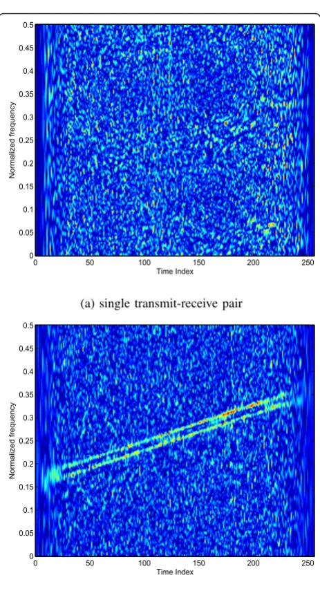
Two different examples are simulated in this section. In the first example, the two targets have close DODs (10° and 15°) observed at the transmitter, whereas their DOAs observed at the receiver have a larger separation (5° and 20°). The parameters of the targets are summar-ized in Table 1. The increasing Doppler signature of each target indicates the target movement towards the transmit and receive arrays in a way that the sum two-way slant range decreases over time.
In Figure 1a we depict the PWVD of the signal corre-sponding to the first receive antenna and the waveform transmitted from the first transmit antenna. The PWVD
averaged over all the NtNr = 24 transmit and receive
antenna combinations is shown in Figure 1b. The input
SNR in this plot is -12 dB. To reduce the sidelobe
interference, a Hamming window of length H= 127 is
used in computing the PWVD. It is evident that, while the TFD auto-terms of the signals are difficult to be recognized in the single transmit-receive antenna pair case because of the presence of a high level of noise, they become clearly identifiable in the sensor averaged TFD due to substantial mitigation of the noise as well as the cross-terms. As discussed in Section 5, cross-terms in the averaged TFD are attenuated according to the varying level of spatial correlation between the respec-tive contributing signal components, whereas the reduc-tion of the noise primarily depends on the number of virtual sensors. The latter, in our case, is the product of the number of transmit antennas and the number of Table 1 Signal parameters of Example 1
Start freq.
End freq.
DOD (deg)
DOA (deg)
Target 1 0.15 0.35 10 5
Target 2 0.17 0.37 15 20
Time Index
Normalized frequency
0 50 100 150 200 250
0 0.05 0.1 0.15 0.2 0.25 0.3 0.35 0.4 0.45 0.5
(a) single transmit-receive pair
Time Index
Normalized frequency
0 50 100 150 200 250
0 0.05 0.1 0.15 0.2 0.25 0.3 0.35 0.4 0.45 0.5
(b) averaged over all virtual sensor pairs
receive antennas. In this example, the spatial correlation coefficient has a high value of 0.956 at the transmit array and a low value of 0.288 at the receive array, resulting in an overall spatial correlation coefficient of the MIMO array at a low level of 0.275 that results in good cross-term suppression. It is noted that, because of the significant cross-term suppression, owing to spatial domain filtering, the two close chirp waveforms can be clearly separated in the time-frequency domain for IF estimation and target discrimination.
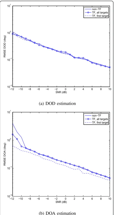
In Figure 2, the root-mean-square error (RMSE) of the DOD and DOA estimation results of the first target are compared for three different scenarios, namely, joint
ESPRIT-MUSIC without the use of time-frequency ana-lysis, time-frequency ESPRIT-MUSIC with all three sig-nals selected for consideration, and time-frequency ESPRIT-MUSIC that only considers the signal corre-sponding to the first target. The results are averaged over 100 independent trials. When both signals are selected in the time-frequency ESPRIT-MUSIC, the per-formance is almost the same as the conventional ESPRIT-MUSIC when the input SNR is moderate or high. While the time-frequency ESPRIT-MUSIC benefits from the SNR enhancement, the performance is never-theless affected by colored noise due to the selection of frequency regions. As has been the case in time-frequency DOA estimation techniques [15,19], the advantage of utilizing time-frequency analysis becomes more pronounced in the underlying example in low SNR scenarios, where the higher-order error terms becomes dominant in the conventional ESPRIT-MUSIC technique. It is interesting to note that, because of the wider separations of the targets in terms of their DOAs, good DOD estimation performance is achieved despite of the small angular separation of the two DODs. Further, by selecting only the first target for joint DOD/ DOA estimation through the time-frequency domain discriminations, the DOA estimation performance is substantially improved, whereas the improvement of the DOD estimation performance is fairly modest.
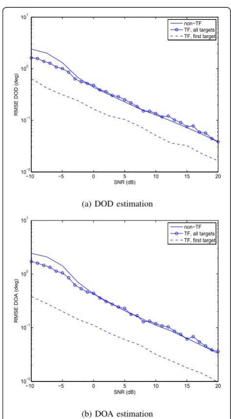
In the second example, the two targets have close DODs (10° and 15°) and close DOAs (15° and 20°). The parameters of the targets are summarized in Table 2. As seen below, the effect of cross-terms in this case is more significant. Therefore, we use two signals of larger Dop-pler frequency difference so as to avoid the effect of cross-terms in auto-term selections.
In Figure 3a we depict the PWVD of the signal corre-sponding to the first receive antenna and the waveform transmitted from the first transmit antenna. The Ham-ming window of length 127 remains the same as in the previous example. Similar to Figure 1a, the signal time-frequency signature cannot be recognized in this plot due to the low input SNR. When averaging the PWVD
over all the NtNr = 24 transmit and receive antenna
combinations, as shown in Figure 3b, the auto-terms are significantly enhanced and can be clearly identified in this plot. The difference between this plot and Figure 1b is also clear in the sense that the residual cross-terms are much higher. In this example, the spatial correlation
−12 −10 −8 −6 −4 −2 0 2 4 6 8 10
10−2 10−1 100 101
SNR (dB)
RMSE DOD (deg)
non−TF TF, all targets TF, first target
(a) DOD estimation
−12 −10 −8 −6 −4 −2 0 2 4 6 8 10
10−2
10−1 100 101
SNR (dB)
RMSE DOA (deg)
non−TF TF, all targets TF, first target
(b) DOA estimation
Figure 2Comparison of RMSE performance.(a)DOD estimation;
(b)DOA estimation.
Table 2 Signal parameters of Example 2
Start freq.
End freq.
DOD (deg)
DOA (deg)
Target 1 0.15 0.35 10 15
coefficient at the transmit array remains 0.956, whereas that at the receive array becomes 0.903 due to the closer angular separation between the two DOAs. This sets the overall spatial correlation coefficient of the MIMO array
to the high value of 0.863. To illustrate the effect of cross-terms on signals with close Doppler signature, Fig-ure 3c plots the averaged PWVD for the chirp signals used in the first example.
In Figure 4, the RMSE of the DOD and DOA estima-tion results of the first target are compared for the same three different scenarios. When both signals are selected, the time-frequency ESPRIT-MUSIC still bene-fits from the SNR enhancement over low SNR regions. The performance of both DOD and DOA estimates is significantly improved through target discrimination by selecting only the first target. This improvement stems from overcoming the close angular separation of the
Time Index
Normalized frequency
0 50 100 150 200 250 0
0.05 0.1 0.15 0.2 0.25 0.3 0.35 0.4 0.45 0.5
(a) single transmit-receive pair
Time Index
Normalized frequency
0 50 100 150 200 250 0
0.05 0.1 0.15 0.2 0.25 0.3 0.35 0.4 0.45 0.5
(b) averaged over all virtual sensor pairs
Time Index
Normalized frequency
0 50 100 150 200 250 0
0.05 0.1 0.15 0.2 0.25 0.3 0.35 0.4 0.45 0.5
(c) averaged PWVD of signals with closer frequency difference of 0.2
Figure 3Comparison of PWVD results.(a)Single transmit-receive pair;(b)averaged over all virtual sensor pairs;(c)averaged PWVD of signals with closer frequency difference of 0.2.
−10 −5 0 5 10 15 20
10−2 10−1
100 101
SNR (dB)
RMSE DOD (deg)
non−TF TF, all targets TF, first target
(a) DOD estimation
−10 −5 0 5 10 15 20
10−2 10−1
100 101
SNR (dB)
RMSE DOA (deg)
non−TF TF, all targets TF, first target
(b) DOA estimation
Figure 4Comparison of RMSE performance.(a)DOD estimation;
targets at both the transmitter and receiver sides using time-frequency signature selections.
7. Conclusions
We have proposed the use of spatial time-frequency dis-tributions (STFDs) for the joint DOD and DOA estima-tion of moving targets in a input multiple-output (MIMO) radar. Time-frequency analysis was applied to the target nonstationary Doppler data to enable signal enhancement and target discrimination. With MIMO configurations, the virtual array provided by the combination of different transmit and receive antenna pairs yields a significant number of virtual sen-sors. The virtually increased aperture empowers the STFD and allows for increased signal-to-noise ratio (SNR) and cross-term suppression, leading to reliable signal identification and selection. This, in turn, improves DOD/DOA estimation of weak targets with a low SNR. Most importantly, it was shown that the cap-ability of discriminating targets with separable Doppler signatures in the time-frequency domain yields signifi-cant performance improvement of DOD/DOA estima-tion for targets with close angular separaestima-tions.
Endnote
a
While joint block diagonalization may yield a better solution for subspace estimation from a set of STFD matrices defined in a region [13], we use weighted time-frequency averaging in this article for simplicity and intuitive description and implementations.
Acknowledgements
The study of Y. D. Zhang and M. G. Amin was supported in part by a subcontract with Dynetics, Inc. for research sponsored by the Air Force Research Laboratory (AFRL) under Contract FA8650-08-D-1303. Part of this study was presented at the 2011 IEEE International Conference on Acoustics, Speech, and Signal Processing, Prague, Czech Republic, May 2011 [27].
Author details
1
Center for Advanced Communications, Villanova University, Villanova, PA 19085, USA2Air Force Research Laboratory, AFRL/RYMD, Dayton, OH 45433,
USA
Competing interests
The authors declare that they have no competing interests.
Received: 16 November 2011 Accepted: 8 May 2012 Published: 8 May 2012
References
1. E Fisher, A Haimovich, R Blum, D Chizhik, L Cimini, R Valenzuela, MIMO radar: an idea whose time has come, inProc IEEE Radar Conf, Philadelphia, PA, pp. 71–78 (2004)
2. Li J, Stoica P (eds.),MIMO Radar Signal Processing(Wiley-IEEE Press, New York, NY, 2009)
3. J Li, P Stoica, MIMO radar with colocated antennas. IEEE Signal Process Mag.25(2), 106–114 (2007)
4. C Duofang, C Baixiao, Q Guodong, Angle estimation using ESPRIT in MIMO radar. Electron Lett.44(2), 770–771 (2008). doi:10.1049/el:20080276
5. M Jin, G Liao, J Li, Joint DOD and DOA estimation for bistatic MIMO radar. Signal Process.89, 244–251 (2009). doi:10.1016/j.sigpro.2008.08.003 6. J Chen, H Gu, W Su, A new method for joint DOD and DOA estimation in
bistatic MIMO radar. Signal Process.90, 714–719 (2010). doi:10.1016/j. sigpro.2009.08.003
7. ML Bencheikh, Y Wang, Joint DOD-DOA estimation using combined ESPRIT-MUSIC approach in MIMO radar. Electron Lett.46(2), 1081–1083 (2010) 8. NJ Willis, HD Griffiths,Advances in Bistatic Radar, (SciTech Publishing,
Raleigh, NC, 2007)
9. Y Zhang, GJ Frazer, MG Amin, Concurrent operation of two over-the-horizon radars. IEEE J Sel Topics Signal Process.1(2), 114–123 (2007) 10. GJ Frazer, Y Abramovich, BA Johnson, Use of adaptive non-causal transmit
beamforming in OTHR: experimental results, inIEEE Radar Conf, Rome, Italy, pp. 311–316 (2008)
11. VC Chen, H Ling,Time-Frequency Transforms for Radar Imaging and Signal Analysis, (Artech House, London, 2002)
12. A Belouchrani, M Amin, Blind source separation based on time-frequency signal representation. IEEE Trans Signal Process.46, 2888–2898 (1998). doi:10.1109/78.726803
13. A Belouchrani, MG Amin, Time-frequency MUSIC. IEEE Signal Proc Lett.6(2), 109–110 (1999)
14. AB Gershman, MG Amin, Wideband direction-of-arrival estimation of multiple chirp signals using spatial time-frequency distributions. IEEE Signal Proc Lett.7(2), 152–155 (2000)
15. Y Zhang, W Mu, MG Amin, Time-frequency maximum likelihood methods for direction finding. J Franklin Inst.337(2), 483–497 (2000)
16. Y Zhang, MG Amin, Spatial averaging of time-frequency distributions for signal recovery in uniform linear arrays. IEEE Trans Signal Process.48(2), 2892–2902 (2000)
17. MG Amin, Y Zhang, Direction finding based on spatial time-frequency distribution matrices. Digital Signal Process.10(2), 325–339 (2000) 18. A Belouchrani, K Abed-Meraim, MG Amin, AM Zoubir, Joint
anti-diagonalization for blind source separation, inProc IEEE Int Conf Acoustics, Speech, and Signal Proc, vol. 5. Salt Lake City, UT, pp. 2789–2792 (2001) 19. Y Zhang, W Mu, MG Amin, Subspace analysis of spatial time-frequency distribution matrices. IEEE Trans Signal Process.49(2), 747–759 (2001) 20. A Hassanien, AB Gershman, MG Amin, Time-frequency ESPRIT for
direction-of-arrival estimation of chirp signals, inProc IEEE Sensor Array and Multichannel Signal Processing Workshop, Rosslyn, VA, pp. 337–341 (2002) 21. W Mu, MG Amin, Y Zhang, Bilinear signal synthesis in array processing. IEEE
Trans Signal Process.51(2), 90–100 (2003)
22. N Linh-Trung, A Belouchrani, K Abed-Meraim, B Boashash, Separating more sources than sensors using time-frequency distributions. EURASIP J Appl Signal Process.2005(2), 2828–2847 (2005)
23. Y Zhang, MG Amin, Blind separation of nonstationary sources based on spatial time-frequency distributions. EURASIP J Applied Signal Processing.
2006, 13 (2006). Article ID 64785
24. MG Amin, Y Zhang, Spatial time-frequency distributions and DOA estimation, inClassical and Modern Direction of Arrival Estimation, ed. by Tuncer E, Friedlander B Academic Press, Burlington, MA, pp. 185–217 (2009) 25. MI Skolnik,Introduction to Radar Systems, 3rd edn. (Mc-Graw Hill, New York,
NY, 2001)
26. L Cohen,Time-Frequency Analysis, (Prentice-Hall, Upper Saddle River, NJ, 1994)
27. YD Zhang, MG Amin, MIMO radar for direction finding with exploitation of time-frequency representations, inProc IEEE Int Conf Acoustics, Speech, and Signal Proc, Plague, Czech Republic, pp. 2760–2763 (2011)
doi:10.1186/1687-6180-2012-102