R E S E A R C H
Open Access
A variable step-size strategy for distributed
estimation over adaptive networks
Muhammad O Bin Saeed, Azzedine Zerguine
*and Salam A Zummo
Abstract
A lot of work has been done recently to develop algorithms that utilize the distributed structure of anad hocwireless sensor network to estimate a certain parameter of interest. One such algorithm is called diffusion least-mean squares (DLMS). This algorithm estimates the parameter of interest using the cooperation between neighboring sensors within the network. The present work proposes an improvement on the DLMS algorithm by using a variable step-size LMS (VSSLMS) algorithm. In this work, first, the well-known variants of VSSLMS algorithms are compared with each other in order to select the most suitable algorithm which provides the best trade-off between performance and complexity. Second, the detailed convergence and steady-state analyses of the selected VSSLMS algorithm are performed. Finally, extensive simulations are carried out to test the robustness of the proposed algorithm under different scenarios. Moreover, the simulation results are found to corroborate the theoretical findings very well.
Keywords: Variable step-size least mean square algorithm; Diffusion least mean square algorithm; Distributed network
1 Introduction
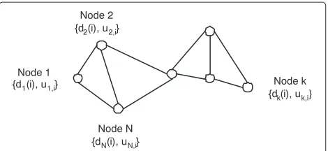
The advent ofad-hocwireless sensor networks has created renewed interest in distributed computing and opened up new avenues for research in the areas of estimation and tracking of parameters of interest where a robust, scal-able, and low-cost solution is required. To illustrate this point clearly, consider a set ofNsensor nodes spread over a wide geographic area, as shown in Figure 1. Each node takes sensor measurements at every sampling instant. The goal here is to estimate a certain unknown parameter of interest using these sensed measurements. In a central-ized network, all nodes transmit their readings to a fusion center where the processing takes place. However, this system is prone to any failure of the fusion center. Fur-thermore, large amounts of energy and communication resources may be required for the complete signal pro-cessing task between the center and the entire network to be successfully carried out. These resources needed could become considerable, as the distance between the nodes and the center increases [1].
Anad hocnetwork, on the other hand, depends on dis-tributed processing with the nodes communicating only
*Correspondence: [email protected]
Electrical Engineering Department, King Fahd University of Petroleum and Minerals, Dhahran 31261, Saudi Arabia
with their neighbors and the processing taking place at the nodes themselves. As no hierarchical structure is involved, any node failure would not result in the failure of the entire network. Extensive research has been done in the field of consensus-based distributed signal processing and resulted in a variety of algorithms [2].
In this work, a brief overview of the virtues and lim-itations of these algorithms [3-10] is conducted, thus providing the background against which our contribution is justified. Incremental algorithms organize the network in a Hamiltonian cycle [3]. The estimation is completed by passing the estimate from node to node, improving the accuracy of the estimate with each new set of data per node. This algorithm is termed the incremental least mean squares (ILMS) algorithm as it uses the LMS algo-rithm [11] with incremental steps within each iteration [3]. A general incremental stochastic gradient descent algorithm was developed in [4], for which [3] can be considered a special case. These algorithms are heavily dependent on the Hamiltonian cycle and in case of a node failure, a new cycle has to be initiated. The problem of reconstructing the cycle is non-deterministic polynomial-time hard [12]. A quantized version of the ILMS algo-rithm was suggested in [5]. A fully distributed algoalgo-rithm was proposed in [6], called diffusion least mean squares
}
Figure 1Adaptive network ofNnodes.
(DLMS) algorithm. In the DLMS algorithm, neighbor nodes share their estimates in order to improve the over-all performance; see also [7]. Ultimately, this algorithm is robust to node failure as the network is not dependent on any single node. On the other hand, the authors in [8] introduced a scheme to adapt the combination weights at each iteration for each node instead of having as fixed weights for the shared data. In this case, the performance is improved if more weight is given to the estimates of the neighbor nodes that are providing more improvement per iteration.
All the previously mentioned algorithms are gener-ally based on a non-constrained optimization technique, except in [8] which uses constrained optimization to adapt the weights only. However, the authors in [9] use the con-straint that all nodes converge to the same steady-state estimate to derive the distributed LMS algorithm. This algorithm is unfortunately hierarchical, thus making it complex and not completely distributed. To remedy this situation, a fully distributed algorithm based on the same constraint was suggested in [10]. The algorithms in [9,10] have been shown to be robust to inter-sensor noise, a property not possessed by the diffusion-based algorithms. However, it has been shown in [7] that diffusion-based algorithms perform better in general.
All the above-mentioned algorithms use a fixed step-size. In general, the step-size is kept the same for all nodes. As a result, the nodes with better signal-to-noise ratio (SNR) may converge quicker and provide a reasonably good performance. However, the nodes with poor SNR will not provide similar performance despite cooperation from neighboring nodes. As a result, a distributed algo-rithm may provide improvement in average performance but individually, some nodes will still not be perform-ing similarly to the other nodes. One solution for this problem was provided by [8]. The work in [8] provides a computationally complex method to improve the per-formance of the DLMS algorithm. For every iteration, an error correlation matrix is formed for each node. A decision is made based on this decision as to the weights of the neighbors. Thus, the combiner weights
are adapted at every iteration according to the perfor-mance of the neighbors of each node. Simulation results from [8] have shown slight improvement in the perfor-mance, but this has been achieved at the cost of high computational complexity.
In comparison, a much simpler solution was sug-gested in [13], using a variable step-size LMS algo-rithm. This resulted in the variable step-size diffusion LMS (VSSDLMS) algorithm. Preliminary results showed remarkable improvement in performance at a reasonably low computational cost. The idea is to vary the step-size at each iteration based on the error performance. Each node will alter its step-size according to its own individual per-formance. As a result, not only the average performance improves remarkably but the individual performances of the nodes also get better.
A different diffusion-based algorithm was proposed in [14] using the recursive least squares (RLS) algorithm to obtain the diffusion RLS (DRLS) algorithm. This DRLS algorithm provided exceptional results in both speed and performance. Another RLS-based distributed estimation algorithm has been studied in [15,16]. The latter algo-rithm is hierarchical in nature, which makes its com-plexity higher than that of the DRLS algorithm. The RLS algorithm is inherently far more complex compared with the LMS algorithm. In this work, it is shown that despite the LMS algorithm being inferior to the RLS algo-rithm, using a variable step-size allows the LMS algorithm to achieve performance very close to that of the RLS algorithm.
In order to achieve better performance, various other algorithms have been proposed in the literature, such as in [17-19]. The works in [17,18] propose distributed Kalman filtering algorithms that provide efficient solutions for several applications. A survey of distributed particle filter-ing is provided in [19]. This work takes a look at several solutions proposed for nonlinear distributed estimation. However, the focus of this work is primarily on LMS-based algorithms, so these algorithms will not be included in any further discussion.
algorithm with similar existing algorithms. Note that the performance of the proposed algorithm is assessed under different conditions. Interestingly, the theoretical find-ings are found to corroborate the simulation results very well. Moreover, a sensitivity analysis is performed on the proposed algorithm.
The paper is organized as follows. Section 2 describes the problem statement and briefly introduces the DLMS algorithm. Section 3 incorporates the VSSLMS algorithm into the DLMS algorithm, and then complete conver-gence and stability analyses are carried out. Simulation results are given in Section 4 followed by a thorough dis-cussion of the results. Finally, Section 5 concludes the work.
Notation.Boldface letters are used for vectors/matrices and normal font for scalar quantities. Matrices are defined by capital letters and small letters are used for vectors. The notation(.)T stands for transposition operation for vec-tors and matrices and expectation operation is denoted by E[.]. Any other mathematical operators that have been used will be defined as they are introduced in the paper.
2 Problem statement
Consider a network of N sensor nodes deployed over a geographical area for estimating an unknown parameter vectorwoof size(M×1), as shown in Figure 1. Each node khas access to a time realization of a known regressor vec-toruk(i)of size(1×M)and a scalar measurementdk(i) that are related by
dk(i)=uk(i)wo+vk(i), 1≤k≤N (1)
where vk(i) is a spatially uncorrelated zero-mean addi-tive white Gaussian noise with varianceσv2
kandidenotes
the time index. The measurements, dk(i) anduk(i), are used to generate an estimate,wk(i)of size(M×1), of the unknown vectorwo. Assuming that each node cooperates only with its neighbors, then each nodek has access to updateswl(i), from itsNk neighbor nodes at every time instant i, wherel∈Nk
l=k , in addition to its own estimate, wk(i). Two different schemes have been introduced in the literature for the diffusion algorithm. The adapt-then-combine (ATC) scheme [7] first updates the local estimate using the adaptive algorithm used and then the interme-diate estimates from the neighbors are fused together. The second scheme, called combine-then-adapt (CTA) [6], reverses the order. It is found that the ATC scheme outperforms the CTA scheme [7] and therefore, this work uses the ATC scheme.
The objective of the adaptive algorithm is to minimize the following global cost function given by
J(w)=
The steepest descent algorithm is given as
wk(i+1)=wk(i)+μ
is the cross-correlation between dk and uk, Ru,k = E
uTkuk
is the auto-correlation of uk, andμ is the step-size. The recursion defined in (3) requires full knowledge of the statistics of the entire net-work. A more practical solution utilizes the distributive nature of the network. The work in [6] gives a fully dis-tributed solution, which has been modified and improved in [7]. The update equation is divided into two steps. The first step performs the adaptation, while the second step combines the intermediate updates from neighbor-ing nodes. The resultneighbor-ing scheme is called
adapt-then-combine or ATC. Using the ATC scheme, the diffusion
LMS algorithm is given as
k(i+1)=wk(i)+μkuk(i)[dk(i)−uk(i)wk(i)]
wk(i+1)=
l∈Nk
clkl(i+1), (4)
wherek(i+1)is the intermediate update,μkis the step-size for nodek, andclk is the weight connecting nodek to its neighboring nodel ∈ Nk, whereNk includes node k, andclk = 1. Further details on the formation of the weightsclkcan be found in [6,7].
3 Variable step-size diffusion LMS algorithm The VSSLMS algorithms show marked improvement over the LMS algorithm at a low computational complex-ity [20-25]. Therefore, this variation is inserted in the distributed algorithm to inherit the improved perfor-mance of the VSSLMS algorithm. Different variations have their own advantages and disadvantages. A com-plex step-size adaptation algorithm would not be suitable because of the physical limitations of the sensor node. As shown in [23], the algorithm proposed by [20] shows the best performance as well as having low complex-ity. Therefore, it is well suited for this application. A further comparison of performance of these variants in the present scenario confirm our choice of the VSSLMS algorithm.
the proposed distributed algorithm. Then the VSSDLMS algorithm is governed by the following:
k(i+1)=wk(i)+μk(i)uk(i) (dk(i)−uk(i)wk(i)),
wheref[μk(i)] is the step-size adaptation function that is defined using the VSSLMS adaptation given in [20] where the update equation is given by
μk(i+1)=αμk(i)+γ (dk(i)−uk(i)wk(i))2 =αμk(i)+γe2k(i), (6)
whereek(i)=dk(i)−uk(i)wk(i), 0< α <1 andγ >0. Since nodes exchange data amongst themselves, their current update will then be affected by the weighted aver-age of the previous estimates. Therefore, to account for this inter-node dependence, it is suitable to study the performance of the whole network. Hence, some new variables need to be introduced and the local ones are transformed into global variables as follows:
w(i)=col{w1(i),. . .,wN(i)},
From these new variables, a completely new set of equations representing the entire network is formed, starting with the relation between the measurements
d(i)=U(i)w(o)+v(i), (7)
where w(o) = Qwo, and Q = col{I
M,IM,. . .,IM} is a MN ×Mmatrix. Similarly, the update equations can be remodeled to represent the entire network
(i+1)=w(i)+D(i)UT(i) (d(i)−U(i)w(i)), onal step-size matrix; and the error energy matrix,E(i), is given by
E(i)=diage21(i)IM,e22(i)IM,. . .,e2N(i)IM . (9)
Considering the above set of equations, the mean and mean-square analyses and the steady-state behavior of the VSSDLMS algorithm are carried out as shown next. The mean analysis considers the stability of the algo-rithm and derives a bound for the step-size which would guarantee convergence. The mean-square analysis also derives transient and steady-state expressions for the mean square deviation (MSD) and the excess mean square error (EMSE). The MSD is defined as the error in the esti-mate of the unknown vector. The weight-error vector for nodekis given by
˜
wk(i)=wo−wk(i), (10)
then the MSD can be simply defined as
MSD=E
Similarly, the EMSE is derived from the error equation as follows:
which can be solved further to get the following expres-sion for the EMSE:
EMSE=E
˜wk(i)2Rk
, (12)
whereRkis the autocorrelation matrix for nodek.
3.1 Mean analysis
To begin with, let us introduce the global weight-error vector defined in [6,26] as
˜
w(i)=w(o)−w(i). (13)
SinceGw(o) = w(o), by incorporating the global weight-error vector into (8), we get
˜
Here we use the assumption that the step-size matrix D(i) is independent of the regressor matrix U(i) [20]. Accordingly, for small values of γ in (6), the following relation holds true asymptotically
where EUT(i)U(i)=RUis the auto-correklation matrix ofU(i), and taking the expectation on both sides of (14) gives
Ew˜(i+1)=G(IMN−E [D(i)]RU)E
˜
w(i), (16)
where the expectation of the second term of the right-hand side of (14) is 0 since the measurement noise is spatially uncorrelated with the regressor and zero-mean, as explained earlier.
From (16), we see that for stability in the mean we must have|λmax(GB)| < 1, where B = (IMN−E [D(i)]RU).
So we can see that the cooperation mode only enhances the stability of the system (for further details, refer to [6,7]). Since stability is also dependent on the step-size, then the algorithm will be stable in the mean if
n
which holds true if the mean of the step-size is governed by
is the maximum eigenvalue of the auto-correlation matrix Ru,k. This scenario is different from that of the fixed step-size as in this case where the system is stable only when the mean of the step-size is within the limits defined by (20).
3.2 Mean-square analysis
In this section, the mean-square analysis of the VSS-DLMS algorithm is investigated. Here, the weighted norm has been used instead of the regular norm. The motiva-tion behind using a weighted norm stems from the fact that even though the MSD does not require a weighted norm, the evaluation of the EMSE depends on a weighted norm. In order to accommodate both these measures, a general analysis is conducted using a weighted norm, where a weighting matrix is replaced by an identity matrix for the case of MSD, where a weighting matrix is not required [26].
We take the weighted norm of (14) and then apply the expectation operator to both of its sides. This yields the following: Using the data independence assumption [26] and applying the expectation operator gives
E
3.2.1 Mean-square analysis for Gaussian data
The evaluation of the expectations in (24) is quite tedious for non-Gaussian data. Therefore, it is assumed here that the data is Gaussian in order to evaluate (24). The auto-correlation matrix can be decomposed asRU = TTT, whereis a diagonal matrix containing the eigenvalues for the entire network and Tis a matrix containing the eigenvectors corresponding to these eigenvalues. Using this eigenvalue decomposition, we define the following relations
¯
w(i)=TTw˜(i) U¯(i)=U(i)T G¯ =TTGT ¯
where the input regressors are considered independent of each other at each node and the step-size matrix D(i) is block-diagonal, so it does not transform since TTT = I. Using these relations, (21) and (24) can be the bvec operator divides the matrix into smaller blocks and then applies the vec operator to each of the smaller blocks. Now, letRv = vIM denote the block diago-nal noise covariance matrix for the entire network, where denotes the block Kronecker product [27] andv is a diagonal noise variance matrix for the network. Hence, the second term of the right-hand side of (25) is
EvT(i)Y¯T(i)¯Y¯(i)v(i)=bT(i)σ¯, (27)
whereb(i)=bvecRvE
D2(i) .
The fourth-order moment EU¯T(i)Y¯T(i)¯Y¯(i)U¯(i)in (26) remains to be evaluated. Using the step-size indepen-dence assumption and theoperator, we get
bvec
where we have from [6]
A=diag{A1,A2,. . .,AN}, (29)
and each matrixAkis given by
Ak=diag
wherekdefines the diagonal eigenvalue matrix andλkis the eigenvalue vector for nodek.
The output of the matrix E [D(i)D(i)] can be written
Now applying the bvec operator to the weighting matrix ¯
Then (21) will take on the following form:
E ¯w(i+1)2σ¯=E
¯w(i)2F(i)σ¯
+bT(i)σ¯, (34)
which characterizes the transient behavior of the network. Although (34) does not explicitly show the effect of the variable step (VSS) algorithm on the network’s perfor-mance, this effect is in fact subsumed in the weighting matrix,F(i) which varies for each iteration, unlike in the fixed step-size LMS algorithm where the analysis shows that this weighting matrix remains fixed at all iterations. Also, (33) clearly shows the effect of the VSS algorithm on the performance of the algorithm through the presence of the diagonal step-size matrixD(i).
3.2.2 Learning behavior of the proposed algorithm
In this section, the learning behavior (which shows how the algorithm evolves with time) of the VSSDLMS algorithm is evaluated. Starting withw0¯ =w(o)andD0= μ0IMN, we have for iteration(i+1)
E(i−1)=diagE ¯w(i−1)2λ+σv,12 IM,. . .,
E [D(i)]=αE [D(i−1)]+γE(i−1) (36)
then incorporating the above relations in (34) gives
E ¯w(i+1)2σ¯=E ¯w(i)2F(i)σ¯+bT(i)σ¯
Now, after subtracting the results of iterationifrom those of iteration(i+1)and simplifying them, we get
E ¯w(i+1)2σ¯=E ¯w(i)2σ¯+w¯(o)2
which can be defined iteratively as
F(i+1)=F(i)F(i), (44)
F(i+1)=F(i)F(i)+bT(i)IMN. (45) In order to evaluate the MSD and EMSE, we need to define the corresponding weighting matrix for each of them. Taking σ¯ = (1/N)bvec{IMN} = qη andη(i) =
The relations in (46) and (47) govern the transient behavior of the MSD and EMSE of the proposed algo-rithm. These relations show how the effect on the pro-posed algorithm’s transient behavior of the weighting matrix varies from one iteration to the next as the weight-ing matrix itself varies at each iteration. This is not the case in the simple fixed step-size DLMS in [6] where the weighting matrix remains constant for all iterations. Since the weighting matrix depends on the step-size matrix, which becomes very small asymptotically, then both the norm and influence of the weighting matrix also become asymptotically small. From the above relations, it is seen that both the MSD and EMSE become very small at steady-state because the weighting matrix itself becomes small at steady-state and these relations will then depend only on the product of the weighting matrices at each iteration.
3.3 Steady-state analysis
From the second relation in (8), it is seen that the step-size for each node is independent of the data received from other nodes. Even though the connectivity matrix, G, does not permit the weighting matrix,F(i), to be eval-uated separately for each node, this is not the case for the determination of the step-size at any node. Here, we define the misadjustment as the ratio of the EMSE to the minimum mean square error. The misadjustment value is used in determining the steady-state performance of the algorithm [11]. Therefore, taking the approach of [20], we first find the misadjustment, as given by
Mk =
0 500 1000 1500 2000 −70
−60 −50 −40 −30 −20 −10 0
iterations
MSD (dB)
Mathews [22]
Mayyas [19] Costa [20]
Kwong [18]
Figure 2MSD for various VSSLMS algorithms applied to the diffusion scheme.
Incorporating these two steady-state relations in (33) yields the steady-state weighting matrix as
Fss = IM2N2−(IMNE [Dss])−(E [Dss]IMN)
+(E [DssDss])A]
GTGT
, (51)
whereDss=diag
μss,kIM .
Thus, the steady-state mean-square behavior is given by
E ¯wss2σ=E ¯wss2Fssσ
+bTssσ, (52)
where bss = RvD2ss and D2ss = diag
μ2ss,kIM
. Now solving (52), we get
E ¯wss2σ=bTssIM2N2−Fss−1σ. (53)
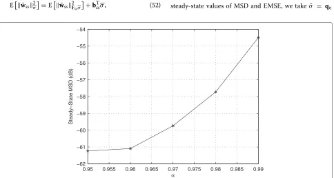
This equation gives the steady-state performance mea-sure for the entire network. In order to solve for the steady-state values of MSD and EMSE, we takeσ¯ = qη
0.95 0.955 0.96 0.965 0.97 0.975 0.98 0.985 0.99
−62 −61 −60 −59 −58 −57 −56 −55 −54
α
Steady−State MSD (dB)
−5 −4.5 −4 −3.5 −3 −2.5 −2 −55
−50 −45 −40 −35 −30 −25 −20 −15 −10 −5
γ (power of 10)
Steady−State MSD (dB)
Figure 4Steady-state MSD values for varying values ofγ.
andσ¯ =λζ, respectively, as in (46) and (47). This gives us the steady-state values for MSD and EMSE as follows:
ηss=bTss
IM2N2−Fss −1
qη, (54)
ζss=bTssIM2N2−Fss −1λ
ζ. (55)
The above two steady-state relationships depend on the steady-state weighting matrix which becomes very small
at state, as explained before. As a result, the steady-state results for the proposed algorithms become very small compared to those for the fixed step-size DLMS algorithm.
4 Numerical results
In this section, several simulation scenarios are consid-ered and discussed to assess the performance of the pro-posed VSSDLMS algorithm. Results have been conducted
0 500 1000 1500 2000
−50 −45 −40 −35 −30 −25 −20 −15 −10 −5 0
DLMS
VSSDLMS−large μ
VSSDLMS−small μ
0 500 1000 1500 2000 −50
−45 −40 −35 −30 −25 −20 −15 −10 −5 0
VSSDLMS−large μ
VSSDLMS−small μ
DLMS
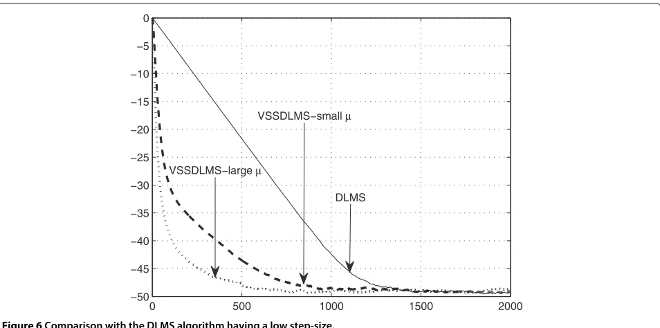
Figure 6Comparison with the DLMS algorithm having a low step-size.
for different average SNR values. The performance mea-sure used throughout these simulations is the MSD. The length of the unknown vector is taken as M = 4. The size of the network is N = 20 nodes. The sensors are randomly placed in an area of 1 unit square. The input regressor vector is assumed to be white Gaussian with auto-correlation matrix having the same variance for all nodes. Results averaged over 100 experiments are shown for the SNR value of 20 dB, a normalized communication range of 0.3, and a Gaussian environment.
First, the discussed that VSSLMS algorithms are com-pared with each other for the case of SNR 20 dB and the results of this comparison are reported in Figure 2. As can be depicted from Figure 2, the algorithm of [20] per-forms the best and is therefore chosen for our proposed VSSDLMS algorithm.
The sensitivity analysis for the selected VSSDLMS algo-rithm operating in the scenario explained above is dis-cussed next. Since the VSSDLMS algorithm depends upon the choice of α andγ, these values are varied to check
0 500 1000 1500 2000
−70 −60 −50 −40 −30 −20 −10 0
iterations
MSD (dB)
NCLMS
DSLMS
DLMSDLMSAC VSSDLMS DRLS
2 4 6 8 10 12 14 16 18 20 −65
−60 −55 −50 −45 −40 −35 −30 −25 −20
Nodes
MSD (dB)
DSLMS NCLMS
DLMS
DLMSAC
VSSDLMS
DRLS
Figure 8MSD at steady-state for 20 nodes and SNR=20 dB.
their effect on the performance of the algorithm. As can be seen from Figure 3, the performance of the VSSDLMS algorithm degrades asα gets larger. Similarly, the perfor-mance of the proposed algorithm improves asγ increases as depicted in Figure 4. This investigation therefore allows for a proper choice ofαandγ to be made.
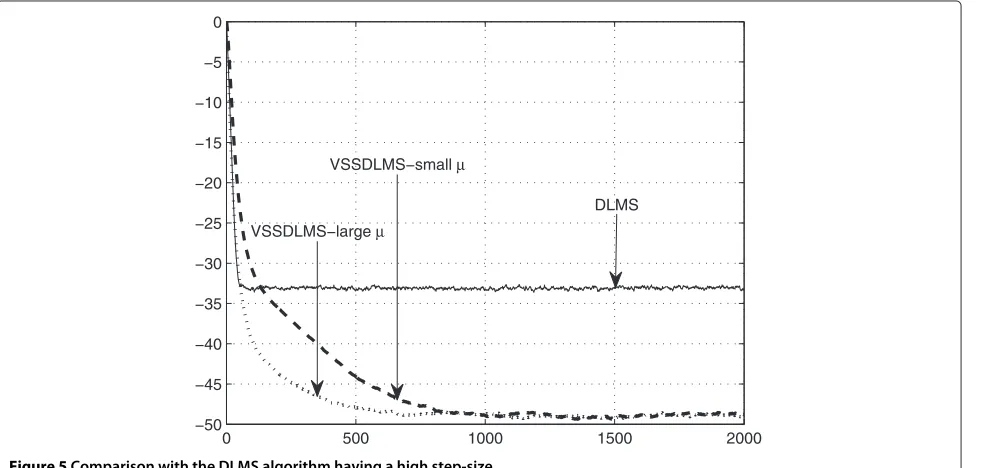
In order to show the importance of varying the step-size, two experiments were run separately. In the first exper-iment, the DLMS algorithm was simulated with a high
step-size while the initial value for the proposed algorithm was kept both low and high. In the second experiment, the step-size of the DLMS algorithm was changed to a low value. As can be seen from Figures 5 and 6, the proposed algorithm converges to the same error floor for both sce-narios. However, the DLMS algorithm converges fast but at a higher error floor in Figure 5. The low value of step-size results in the DLMS algorithm converging at the same error floor as the proposed algorithm but very slowly.
0 500 1000 1500 2000 2500 3000 3500
−50 −45 −40 −35 −30 −25 −20 −15 −10 −5 0
iterations
MSD(dB)
Theory Simulation
0 500 1000 1500 2000 2500 −40
−35 −30 −25 −20 −15 −10 −5 0 5
iterations
MSD(dB)
Theory Simulation
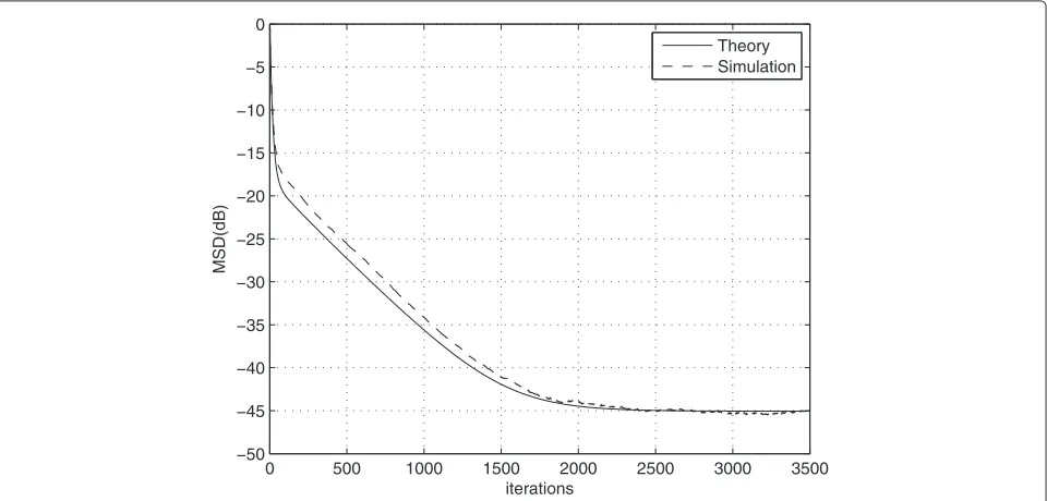
Figure 10Theoretical and simulated MSD withα=0.995 andγ =0.001.
Thus, the proposed algorithm provides fast convergence as well as better performance.
Next, the proposed algorithm is compared with some key existing algorithms, which are the no-cooperation LMS, the distributed LMS [10], the DLMS [6], the DLMS with adaptive combiners (DLMSAC) [8] and the DRLS [14]. Figure 7 reports the performance behavior of these different algorithms. As can be seen from this figure, the
performance of the proposed VSSDLMS algorithm is second only that of the DRLS algorithm. However, the gap in performance is narrow. These results show that when compared with other algorithms of similar com-plexity, the VSSDLMS algorithm exhibits a significant improvement in performance. A similar performance in the steady-state behavior of the proposed VSSDLMS algorithm is obtained as shown in Figure 8. As expected,
0 200 400 600 800 1000
−60 −50 −40 −30 −20 −10 0
iterations
MSD (dB)
VSSDLMS−Full
DLMS−Full
VSSDLMS−2 VSSDLMS−1
DLMS−2 DLMS−1
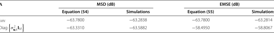
Table 1 Steady-state values for MSD and EMSE
MSD (dB) EMSE (dB)
Equation (54) Simulations Equation (55) Simulations
IMN −63.7800 −63.2838 −63.7800 −63.2814
Diagσu2,kIM
−63.3310 −63.5882 −58.4950 −58.8067
the DRLS algorithm performs better than all other algo-rithms included in this comparison, but the proposed algorithm remains second only to the DRLS algorithm in the steady-state mode. Also, the diffusion process can be appropriately viewed as an efficient and indirect way of adjusting the step-size in all neighboring nodes, which resulted in keeping the steady-state MSD for all nodes nearly the same for all cases.
Next, the comparison between the results predicted by the theoretical analysis of the proposed algorithm and the simulation results is reported in Figures 9 and 10. As can be seen from these figures, the simulation analysis corrob-orates the theoretical findings very well. This is done for a network of 15 nodes withM= 2 and a communication range of 0.35. Two values forα, namelyα = 0.995 and α=0.95, are chosen whereasγ =0.001.
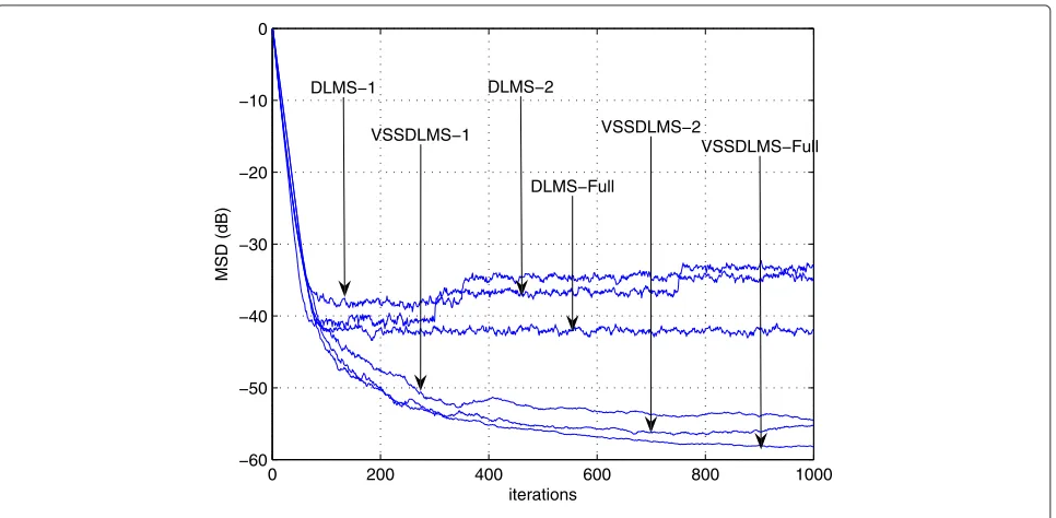
An important aspect of working with sensor nodes is the possibility of a node switching off. In such a case the network may be required to adapt itself. The diffusion scheme is robust to such a change, and this scenario has been considered here and results are shown in Figure 11. A network of 50 nodes is chosen so that enough nodes can be switched off in order to study the performance of the proposed algorithm in this scenario. Two cases are considered. In the first case, 15 nodes are turned off after 50 iterations and then a further 15 nodes are switched off after 300 iterations. In the second case, 15 nodes are switched off after 250 iterations and the next 15 nodes are switched off after 750 iterations. In both cases, the performance degrades initially but recovers to give a sim-ilar performance to the case where there are no nodes being switched off. The difference between the best and worst case scenarios is only about 2 dB. For the DLMS algorithm, however, the performance is worse off the ear-lier the nodes are switched off. The difference between the best and worst case scenarios is almost 9 dB, which further enhances the robustness of the proposed algorithm.
Finally, the comparison between the theoretical and simulated steady-state values for the MSD and EMSE for two different input regressor auto-correlation matri-ces is given in Table 1. As can be seen from this table, a close agreement between theory and simulations has been obtained.
5 Conclusions
The proposed variable step-size diffusion LMS (VSS-DLMS) algorithm has been discussed in detail. Several
popular VSSLMS algorithms are investigated and the algorithm providing the best trade-off between complex-ity and performance is chosen as the proposed VSSDLMS algorithm. Complete convergence and steady-state anal-yses have been carried out to assess the performance of the proposed algorithm. Simulations have been carried out under different scenarios and with different SNR val-ues. A sensitivity analysis has been carried out through extensive simulations. Based on the results of this analysis, the values for the parameters of the VSSLMS algorithm were chosen. The proposed algorithm has been compared with existing algorithms of similar complexity and it has been shown that the proposed algorithm performed sig-nificantly better. Theoretical results were also compared with simulation results and the two were found to be in close agreement with each other. The proposed algo-rithm was then tested under different scenarios to assess its robustness. Finally, a steady-state comparison between theoretical and simulated results was carried out and tab-ulated and the results were also found to be in close agreement with each other.
Competing interests
The authors declare that they have no competing interests.
Acknowledgements
This research work is funded by King Fahd University of Petroleum and Minerals (KFUPM) under research grants FT100012 and RG1112-1&2.
Received: 15 July 2013 Accepted: 26 July 2013 Published: 6 August 2013
References
1. D Estrin, L Girod, G Pottie, M Srivastava, Instrumenting the world with wireless sensor networks, inProceedings of the ICASSP(Salt Lake City, 07–11 May 2001), pp. 2033–2036
2. R Olfati-Saber, JA Fax, RM Murray, Consensus and cooperation in networked multi-agent systems. Proc. IEEE.95(1), 215–233 (2007) 3. CG Lopes, AH Sayed, Incremental adaptive strategies over distributed
networks. IEEE Trans. Signal Process.55(8), 4064–4077 (2007) 4. SS Ram, A Nedic, VV Veeravalli, Stochastic incremental gradient descent
for estimation in sensor networks, inProceedings of the 41st Asilomar Conference on Signals, Systems and Computers(Pacific Grove, 4–7 November 2007), pp. 582–586
5. A Rastegarnia, MA Tinati, A Khalili, Performance analysis of quantized incremental LMS algorithm for distributed adaptive estimation. Signal Process.90(8), 2621–2627 (2010)
6. CG Lopes, AH Sayed, Diffusion least-mean squares over adaptive networks: formulation and performance analysis. IEEE Trans. Signal Process.56(7), 3122–3136 (2008)
7. F Cattivelli, AH Sayed, Diffusion LMS strategies for distributed estimation. IEEE Trans. Signal Process.58(3), 1035–1048 (2010)
9. ID Schizas, G Mateos, GB Giannakis, Distributed LMS for consensus-based in-network adaptive processing. IEEE Trans. Signal Process.57(6), 2365–2382 (2009)
10. G Mateos, ID Schizas, GB Giannakis, Performance analysis of the consensus-based distributed LMS algorithm. EURASIP J. Adv. Signal Process (2009). doi:10.1155/2009/981030
11. S Haykin,Adaptive Filter Theory, 4th edn. (Prentice-Hall, Englewood Cliffs, 2000)
12. CH Papadimitriou,Computational Complexity(Addison-Wesley, Reading, MA, 1993)
13. MO BinSaeed, A Zerguine, SA Zummo, Variable step size least mean square algorithms over adaptive networks, inProceedings of ISSPA 2010 (Kuala Lampur, 10–13 May 2010), pp. 381–384
14. FS Cattivelli, CG Lopes, AH Sayed, Diffusion recursive least-squares for distributed estimation over adaptive networks. IEEE Trans. Signal Process.
56(5), 1865–1877 (2008)
15. G Mateos, ID Schizas, GB Giannakis, Distributed recursive least-squares for consensus-based in-network adaptive estimation. IEEE Trans. Signal Process.57(11), 4583–4588 (2009)
16. G Mateos, GB Giannakis, Distributed recursive least-squares: stability and performance analysis. IEEE Trans. Signal Process.60(7), 3740–3754 (2012) 17. F Cattivelli, AH Sayed, Diffusion strategies for distributed Kalman filtering and smoothing. IEEE Trans. Automatic Control.55(9), 2069–2084 (2010) 18. R Olfati-Saber, Distributed Kalman filtering for sensor networks, in
Proceedings of IEEE CDC 2007(New Orleans, 12–14 December 2007), pp. 5492–5498
19. O Hlinka, F Hlawatsch, PM Djuric, Distributed particle filtering in agent networks: a survey, classification, and comparison. IEEE Signal Proc. Mag.
30(1), 61–81 (2013)
20. RH Kwong, EW Johnston, A variable step size LMS algorithm. IEEE Trans. Signal Process.40(7), 1633–1642 (1992)
21. T Aboulnasr, K Mayyas, A robust variable step-size LMS-type algorithm: analysis and simulations. IEEE Trans. Signal Process.45(3), 631–639 (1997) 22. MH Costa, JCM Bermudez, A robust variable step-size algorithm for LMS
adaptive filters, inProceedings of the ICASSP(Toulouse, 14–19 May 2006), pp. 93–96
23. CG Lopes, JCM Bermudez, Evaluation and design of variable step size adaptive algorithms, inProceedings of the ICASSP(Salt Lake City, 7–11 May 2001), pp. 3845–3848
24. VJ Mathews, Z Xie, A stochastic gradient adaptive filter with gradient adaptive step size. IEEE Trans. Signal Process.41(6), 2075–2087 (1993) 25. AI Sulyman, A Zerguine, Convergence and steady-state analysis of a
variable step-size NLMS algorithm. Signal Process.83(6), 1255–1273 (2003) 26. AH Sayed,Fundamentals of Adaptive Filtering(Wiley, New York, 2003) 27. RH Koning, H Neudecker, T Wansbeek, Block Kronecker products and the
vecb operator. Economics Department, Institute of Economics Research, University of Groningen, Groningen, The Netherlands, Research Memo no. 351, 1990
doi:10.1186/1687-6180-2013-135
Cite this article as:Bin Saeedet al.:A variable step-size strategy for dis-tributed estimation over adaptive networks.EURASIP Journal on Advances in Signal Processing20132013:135.
Submit your manuscript to a
journal and benefi t from:
7 Convenient online submission 7 Rigorous peer review
7 Immediate publication on acceptance 7 Open access: articles freely available online 7 High visibility within the fi eld
7 Retaining the copyright to your article