doi: 10.11648/j.cse.20180201.13
Numerical Method of a Class of Stochastic Delay Population
Models
Changyou Wang
1, 2, *, Kaixiang Yang
1, Xingcheng Pu
1, Rui Li
11
College of Automation, Chongqing University of Posts and Telecommunications, Chongqing, P. R. China
2
College of Applied Mathematics, Chengdu University of Information Technology, Chengdu, P. R. China
Email addresses:
*
Corresponding author
To cite this article:
Changyou Wang, Kaixiang Yang, Xingcheng Pu, Rui Li. Numerical Method of a Class of Stochastic Delay Population Models. Control Science and Engineering. Vol. 2, No. 1, 2018, pp. 27-35. doi: 10.11648/j.cse.20180201.13
Received: December 1, 2018; Accepted: December 19, 2018; Published: January 14, 2019
Abstract:
Our aim in this paper is to present the design and implementation of a new numerical method to solve a class of stochastic delay population models. Firstly, a stochastic predator-prey model with time-delay and white noise is established. And then, a numerical simulation method based on the Milstein method is proposed to simulate the stochastic population model. Finally, the numerical solutions of the population model are obtained by using MATLAB software. The simulation results show that the new numerical simulation method can truly reflect the persistence and extinction process of stochastic predator-prey model, and provide a reference for solving the numerical simulation of the similar population models.Keywords: Time-Delay, White Noise, Stochastic Population Model, Numerical Simulation
1. Introduction
The living environment of biological populations is affected by human activities and environmental changes, and the influence of environmental noise on the living environment of the population cannot be ignored, which has attracted the attention of biologists and has become a new research direction. Maja Vasilova [1] studied the stochastic Gilpin-Ayala predator-prey system with time-varying delays, and obtained the long-term gradual progress, mean estimation and population extinction of the system. Miljana Jovanovic and MajaVasilova [2] studied the non-autonomous stochastic Gilpin-Ayala competition system with time-varying delays, and obtained the conditions of population extinction, non-sustained survival, average persistent survival and weak persistent survival. Aadil Lahrouz and Adel Sufficient Settati [3] gave the necessary and sufficient conditions which guarantee the permanence of a stochastic disturbance SIRS system. Zhang [4] established a stochastic predator-prey model with time delay and predator diffusion, and discussed the existence of a unique global positive solution, the conditions for population extinction and average persistence. In 2017, Zhang et al [5]
proposed a stochastic non-autonomous Lotka–Volterra predator–prey model with impulsive effects, and proved the system has an unique periodic solution which is globally attractive, the persistence and extinction of each species.
In the existing literature describing population dynamics randomization, it is often assumed that the intrinsic growth rate is the most sensitive parameter [6-8] to study the model. In general, it is assumed that the population grows in an environment where ambient noise is the main interfering rate of intrinsic growth, so that the intrinsic growth rate is described as an average plus an error term. At the same time, the well-known central limit theorem pointed out that the error term obeys a normal distribution. In a relatively short time, can use σiB tɺi( ) replace this error term, where σi is the stochastic interference intensity of the population and B tɺi( ) is the standard white noise. That is, the B tɺi( ) is Brownian motion defined on the complete probability space ( , , )Ω F P . If still use
i
12
1 11 1 1
21
2 22 2 2
( )
[ ( ) ( ) ] ( ) ( ),
1 ( ) ( ) ( )
[ ( ) ( ) ] ( ) ( ).
1 ( ) ( )
a t y
dx x r t a t x dt t xdB t
t x t y
a t x
dy y r t a t y dt t ydB t
t x t y
σ β γ σ β γ = − − + + + = − + − + + + (1)
However, to the best of the authors’ knowledge, to this day, still less scholars consider the stochastic multiple populations ecological model with delays. Motivated by the above works, this paper proposes a stochastic three-species predator-prey model with time-delay and white noise, and explore the application of MATLAB soft in solving the numerical solution of the stochastic population model. The rest of this paper is organized as follows: In Section 2, a stochastic predator-prey model is proposed. The numerical solutions of the model are obtained in Section 3. The conclusion is given in the Section 4.
2. Built of Model
Competition-cooperation is a common inter-relationship
among populations in the ecosystem. Many scholars have achieved certain results in the research of such models [10-15]. In nature, the impact of environmental noise on biological populations is also crucial. When the ambient noise is large enough, the population may even be extinct. The biological population simulation with environmental noise is closer to the real situation. At the same time, the lag caused by the pregnancy of biological populations is ubiquitous in the ecosystem, and the differential equation model with time delay has more complex dynamic behavior than the general differential equation model. Considering these factors, this paper proposes a three-species predator-prey models with delays and white noise, in which the two prey populations compete with each other. The stochastic three-species predator-prey model is as follows:
13 3
1 1 1 11 1 1 12 2 2 1 1 1
1 3
23 3
2 2 2 21 1 1 22 2 2 2 2 2
2 3
31 1
3 3 3
1 3
( )
( ) ( )[ - ( - ) - ( - ) - ] ( ) ( ),
1 ( ) ( )
( )
( ) ( )[ - ( - ) - ( - ) - ] ( ) ( ),
1 ( ) ( )
( )
( ) (
)[-1 ( ) (
a x t
dx t x t r a x t a x t dt x t dB t
x t x t
a x t
dx t x t r a x t a x t dt x t dB t
x t x t
a x t
dx t x t r
x t x
τ τ σ β γ τ τ σ β γ β γ = + + + = + + + = +
+ + 32 2 3 3 3
2 3
( )
] ( ) ( ),
) 1 ( ) ( )
a x t
dt x t dB t
t βx t γx t σ
+ + + + (2)
where x t1( ) and x t2( ) are prey populations, x t(3 ) is a predator population, x ti( ) (i=1, 2, 3) is the population density of the three populations at the moment t ,
( 1, 2) i
r i= represents the natural growth rates of the prey populations, r t3( ) is the death rate of the predator
population. a iii( =1, 2) represents the competition loss within the population, a12 and a21 represents the
competitive loss between the population x t1( ) and the population x t2( ), a13 and a23 represents the predation parameter of the population x t3( ) versus the population
1( )
x t and x t2( ) , a31 and a32 represents the
transformation parameter of population x t3( ) predator population x t1( ) andx t2( ). The B tɺi( ) is Brownian motion defined on the complete probability space ( , , )Ω F P .
In the stochastic population model, it is usually assumed that the birth rate and mortality of the population are stochastic. Such a solution no longer approaches a stable positive equilibrium state, but fluctuates at a certain average value. Therefore, studying population extinction and persistent survival becomes a core issue with a stochastic perturbation population model. Below the Milstein method
will be used to numerically simulate the persistence and extinction of the model.
3. Numerical Simulation
In this section, The Milstein numerical simulation method [16-19] will be used to solve the numerical solutions for the models (2). Firstly, the Milstein method will be introduced. Considering the autonomous scalar stochastic differential equation SDE:
0 0 0
( ) ( ( )) ( ( )) ( ),
( ) ( [ , ]),
dy t f y t dt g y t dw t
y t y t t T
= +
= ∈
(3)
where f y( )and ( )g y are continuous measurable functions on
0
[ , ]t T , respectively called offset coefficient and diffusion coefficient,y∈R w t, ( ) is a standard wiener process, and its increment
( ) ( ) ( )
w t w t h w t
∆ = + − (4)
follows a normal distribution N(0, )h . The explicit Milstein m
2
1 ( ) ( ) [ ] (( ) ) / 2.
n n n n n n n
When the parameters in the model (2) take different values, the numerical solutions are obtained for the models (2), respectively, which are shown in Figure 1 to Figure 6.
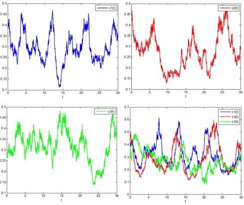
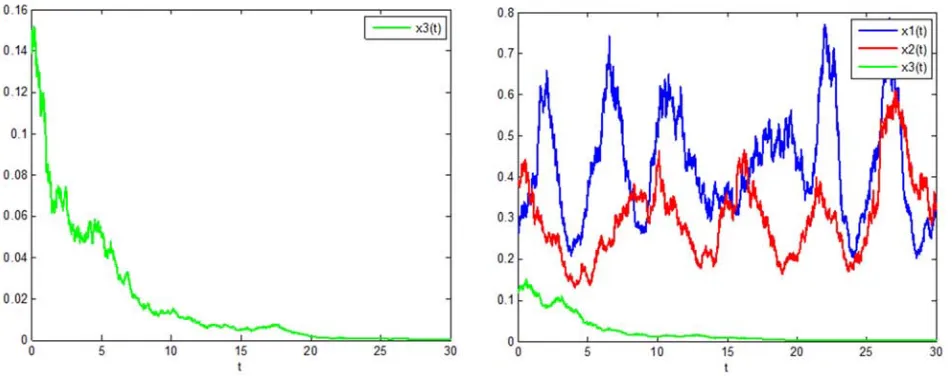
In Figure 1, the parameters are taken as follows:
1 2 3 11 22 12 21 13 23 31 32
1 2 3
1.2, 1, 0.4, 2.5, 1.5, 0.5, 1.2, 1.2, 1, 0.8, 1.5, 0.02.
r r r a a a a a a a a
σ σ σ
= = = = = = = = = = =
= = =
The Milstein method is used to process the stochastic items, and the system persistence time series graph under stochastic disturbance is obtained, and shown in Figure 1.
Figure 1. System persistence time series diagram under stochastic perturbation.
From the Figure 1, it can be seen that under stochastic disturbance, the three species survive continuously, and the
1
x and x2 populations compete with each other and are
restricted by the population x3. Due to the influence of the time-delay, their trends are roughly the same, only delayed in time. When the density x3 of the predator population
density increases, the densities x1 and x2 of prey populations are decreasing. After that, the density of the predator populationx3decreases, and the densitiesof the prey
populations x1 and x2 increase. Repeatedly. Figure 1
reflects these features very well.
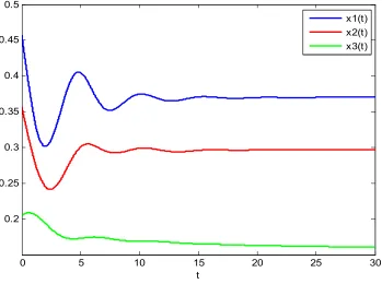
1 2 3 11 22 12 21 13 23 31 32
1 2 3
1.2, 1, 0.5, 2.5, 1.5, 0.5, 1.2, 1.2, 1, 0.8, 1.5, 0.
r r r a a a a a a a a
σ σ σ
= = = = = = = = = = =
= = =
The system persistence time series graph of the determined model is obtained without considering stochastic interference, which is shown in Figure 2.
Figure 2. System persistence time series graph of the determined model.
From the Figure 2, it can be seen that in the absence of stochastic interference, the population density curves of the three species are relatively smooth. Due to the influence of time lag, the trends of x1 and x2 populations are roughly the same, but there is a delay in time. After a short period of volatility, three populations tend to balance and no longer volatility, which is obviously not in line with the laws of biological population changes in nature.
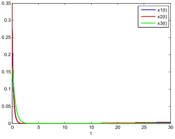
In Figure 3, the parameters are taken as follows:
1 2 3 11 22 12 21 13 23 31 32
1 2 3
0.45, 0.35, 3, 1.3, 2.3, 2.5, 1.2, 7, 8, 1.8, 1.5, 0.2.
r r r a a a a a a a a
σ σ σ
= = = = = = = = = = =
= = =
The system extinction time series graph under stochastic interference is obtained, which is shown in Figure 3.
0 5 10 15 20 25 30
0.2 0.25 0.3 0.35 0.4 0.45 0.5
t
Figure 3. System extinction time series graph under stochastic disturbance.
From the Figure 3, the stochastic disturbances also affect the extinction of biological populations. Due to the effect of stochastic disturbances, the density of biological populations is also fluctuating in the trend of decline, which is in line with natural laws and the species are eventually extinct.
In Figure 4, the parameters are taken as follows:
1 2 3 11 22 12 21 13 23 31 32
1 2 3
0.1, 0.12, 2, 3, 8, 8, 3.5, 2, 2.5, 3.8, 1.8, 0.
r r r a a a a a a a a
σ σ σ
= = = = = = = = = = =
= = =
The system extinction time series graph of the determined model is obtained without considering stochastic interference, which is shown in Figure 4.
Figure 4. System extinction time series graph of the determined model.
From the Figure 4, it can be seen that in the absence of random interference, the population density curves of the three species are vertically decreased until extinct and there is no fluctuation trend. Obviously, the system with stochastic interference is more scientific.
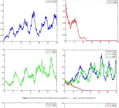
In Figure 5, the parameters are taken as follows:
1 2 3 11 22 12 21 13 23 31 32
1 2 3
1.5, 1.3, 1.1, 1.1, 2.3, 2.5, 1.2, 2.5, 2.5, 3.8, 1.8, 0.02.
r r r a a a a a a a a
σ σ σ
= = = = = = = = = = =
= = =
0 5 10 15 20 25 30 0
0.05 0.1 0.15 0.2 0.25 0.3 0.35
t
The extinction time series graph of the system prey population x2 under stochastic interference is obtained, which is
shown in Figure 5.
Figure 6. Extinction time series graph of predator population x under stochastic disturbance. 3
From the Figure 6, it can be seen that under the action of stochastic disturbances, the predator populations x3 is
extinct, and the prey population x1 and x2 are living in
the system together.
From Figures 1-6, it is obvious that the stochastic disturbances items have influence both on the permanence of the original system. Therefore, in some ecosystems, some species can be controlled to maintain the balance and sustainable development of the ecosystem, and this is also the practical significance of this topic.
According to the data in Figure 1, the code for writing stochastic items using the Milstein method is as follows:
Code 1 clc;
x1=cell(1,1); x2=cell(1,1); x3=cell(1,1);
x1{1}(1)=sin(-0.3*rand)+0.5; x2{1}(1)=sin(-0.3*rand)+0.5; x3{1}(1)=sin(-0.4*rand)+0.5; h=0.01;
tend=30; tau1=1; tau2=2; t=0; k=1;
while t<=tend
x1{1}(k+1)=x1{1}(k)+h*x1{1}(k)*(1.2-2.5*x1{1}(max(1 ,k-tau1/h))-0.5*x2{1}(max(1,k-tau2/h))-(1.2*x3{1}(k)/(1+x1 {1}(k)+x3{1}(k))))+0.02*x1{1}(k)*randn+0.02^2*0.5*x1{1 }(k)*(randn^2-h);
x2{1}(k+1)=x2{1}(k)+h*x2{1}(k)*(1-1.2*x1{1}(max(1,k -tau1/h))-1.5*x2{1}(max(1,k-tau2/h))-(1*x3{1}(k)/(1+x2{1} (k)+x3{1}(k))))+0.02*x2{1}(k)*randn+0.02^2*0.5*x2{1}(k )*(randn^2-h);
x3{1}(k+1)=x3{1}(k)+h*x3{1}(k)*(-0.4+(0.8*x1{1}(k)/( 1+x1{1}(k)+x3{1}(k)))+(1.5*x2{1}(k)/(1+x2{1}(k)+x3{1}( k))))+0.02*x3{1}(k)*randn+0.02^2*0.5*x3{1}(k)*(randn^2-h);
k=k+1; t=t+h; end
tt=(0:h:tend);
plot(tt,x1{1},'b','linewidth',2) hold on
plot(tt,x2{1},'r','linewidth',2) hold on
plot(tt,x3{1},'g','linewidth',2) xlabel('t');
legend('x1(t)', 'x2(t)', 'x3(t)'); hold on
According to the data in Figure 2, some of the code 1 are modified as follows:
x1{1}(k+1)=x1{1}(k)+h*x1{1}(k)*(1.2-2.5*x1{1}(max(1 ,k-tau1/h))-0.5*x2{1}(max(1,k-tau2/h))-(1.2*x3{1}(k)/(1+x1 {1}(k)+x3{1}(k))))
x2{1}(k+1)=x2{1}(k)+h*x2{1}(k)*(1-1.2*x1{1}(max(1,k -tau1/h))-1.5*x2{1}(max(1,k-tau2/h))-(1*x3{1}(k)/(1+x2{1} (k)+x3{1}(k))))
x3{1}(k+1)=x3{1}(k)+h*x3{1}(k)*(-0.5+(0.8*x1{1}(k)/( 1+x1{1}(k)+x3{1}(k)))+(1.5*x2{1}(k)/(1+x2{1}(k)+x3{1}( k))))
According to the data in Figure 3, some of the code 1 are modified as follows:
x1{1}(k+1)=x1{1}(k)+h*x1{1}(k)*(0.45-1.3*x1{1}(max( 1,k-tau1/h))-2.5*x2{1}(max(1,k-tau2/h))-(7*x3{1}(k)/(1+x1 {1}(k)+x3{1}(k))))+0.2*x1{1}(k)*randn+0.2^2*0.5*x1{1}( k)*(randn^2-h);
x2{1}(k+1)=x2{1}(k)+h*x2{1}(k)*(0.35-1.2*x1{1}(max( 1,k-tau1/h))-2.3*x2{1}(max(1,k-tau2/h))-(8*x3{1}(k)/(1+x2 {1}(k)+x3{1}(k))))+
0.2*x2{1}(k)*randn+0.2^2*0.5*x2{1}(k)*(randn^2-h); x3{1}(k+1)=x3{1}(k)+h*x3{1}(k)*(-3+(1.8*x1{1}(k)/(1+ x1{1}(k)+x3{1}(k)))+(1.5*x2{1}(k)/(1+x2{1}(k)+x3{1}(k)) ))+ 0.2*x3{1}(k)*randn+0.2^2*0.5*x3{1}(k)*(randn^2-h);
According to the data in Figure 4, some of the code 1 are modified as follows:
-tau1/h))-8*x2{1}(max(1,k-tau2/h))-(2*x3{1}(k)/(1+x1{1}(k )+x3{1}(k)))); x2{1}(k+1)=x2{1}(k)+h*x2{1}(k)*(0.12-3.5*x1{1}(max( 1,k-tau1/h))-8*x2{1}(max(1,k-tau2/h))-(2.5*x3{1}(k)/(1+x2 {1}(k)+x3{1}(k)))); x3{1}(k+1)=x3{1}(k)+h*x3{1}(k)*(-2+(3.8*x1{1}(k)/(1+ x1{1}(k)+x3{1}(k)))+(1.8*x2{1}(k)/(1+x2{1}(k)+x3{1}(k)) ));
According to the data in Figure 5, some of the code 1 are modified as follows:
x1{1}(k+1)=x1{1}(k)+h*x1{1}(k)*(1.5-1.1*x1{1}(max(1 ,k-tau1/h))-2.5*x2{1}(max(1,k-tau2/h))-(2.5*x3{1}(k)/(1+x1 {1}(k)+x3{1}(k))))+0.02*x1{1}(k)*randn+0.02^2*0.5*x1{1 }(k)*(randn^2-h); x2{1}(k+1)=x2{1}(k)+h*x2{1}(k)*(1.3-1.2*x1{1}(max(1 ,k-tau1/h))-2.3*x2{1}(max(1,k-tau2/h))-(2.5*x3{1}(k)/(1+x2 {1}(k)+x3{1}(k))))+0.02*x2{1}(k)*randn+0.02^2*0.5*x2{1 }(k)*(randn^2-h); x3{1}(k+1)=x3{1}(k)+h*x3{1}(k)*(-1.1+(3.8*x1{1}(k)/( 1+x1{1}(k)+x3{1}(k)))+(1.8*x2{1}(k)/(1+x2{1}(k)+x3{1}( k))))+0.02*x3{1}(k)*randn+0.02^2*0.5*x3{1}(k)*(randn^2-h);
According to the data in Figure 6, some of the code 1 are modified as follows:
x1{1}(k+1)=x1{1}(k)+h*x1{1}(k)*(1.2-2.5*x1{1}(max(1 ,k-tau1/h))-0.5*x2{1}(max(1,k-tau2/h))-(1.2*x3{1}(k)/(1+x1 {1}(k)+x3{1}(k))))+0.02*x1{1}(k)*randn+0.02^2*0.5*x1{1 }(k)*(randn^2-h); x2{1}(k+1)=x2{1}(k)+h*x2{1}(k)*(1-1.2*x1{1}(max(1,k -tau1/h))-1.5*x2{1}(max(1,k-tau2/h))-(1*x3{1}(k)/(1+x2{1} (k)+x3{1}(k))))+ 0.02*x2{1}(k)*randn+0.02^2*0.5*x2{1}(k)*(randn^2-h); x3{1}(k+1)=x3{1}(k)+h*x3{1}(k)*(-0.8+(0.8*x1{1}(k)/( 1+x1{1}(k)+x3{1}(k)))+(1.5*x2{1}(k)/(1+x2{1}(k)+x3{1}( k))))+ 0.02*x3{1}(k)*randn+0.02^2*0.5*x3{1}(k)*(randn^2-h);
4. Conclusion
This paper presents the design and implementation of a new numerical method to solve a class of stochastic delay population models. This method is a powerful tool for solving various population models and can also be applied to other nonlinear differential equations in mathematical physics. Computations are performed using the software package MATLAB7.0. The simulation results show that the new numerical simulation method can truly reflect the persistence and extinction process of stochastic predator-prey model.
Acknowledgements
This work is supported by the Sichuan Science and Technology Program (Grant no. 2018JY0480) of China, the Natural Science Foundation Project of CQ CSTC (Grant no. cstc2015jcyjBX0135) of China, and the National Nature Science Fund (Project no. 61503053) of China.
References
[1] M. Vasilova, Asymptotic behavior of a stochastic Gilpin-Ayala predator-prey system with time-dependent delay, Mathematical and Computer Modelling, 57 (2013) 764-781.
[2] M. Jovanović, M. Vasilova, Dynamics of non-autonomous stochastic Gilpin-Ayala competition model with time-varying delays, Applied Mathematics and Computation, 219 (2013) 6946-6964.
[3] A. Lahrouz, A. Settati, Necessary and sufficient condition and persistence of SIRS system with random perturbation, Applied Mathematics and Computation, 233 (2014) 10-19.
[4] S. Zhang, Random predator-prey system with time delay and diffusion (in Chinese), Acta Matematica Scientia, 35A (2015) 592-603.
[5] S. Zhang, X. Meng, T. Feng, T. Zhang, Dynamics analysis and numerical simulations of a stochastic non-autonomous predator-prey system with impulsive effects, Nonlinear Analysis: Hybrid Systems, 26 (2017) 19-37.
[6] M. Liu, K. Wang, Persistence and extinction of a stochastic single-specie model under regime switching in a polluted environment, Journal of theoretical biology, 264 (2010) 934-944. [7] M. Liu, K. Wang, Global stability of a nonlinear stochastic predator-prey system with Beddington- DeAngefis functional response, Communications in Nonlinear Science and Numerical Simulation, 16 (2011) 1114-1121.
[8] M. Liu, K. Wang, Q. Wu, Survival analysis of stochastic competitive models in a polluted environment and stochastic competitive exclusion principle, Bulletin of Mathematical Biology, 73 (2011) 1969-2012.
[9] Y. Wang, Population dynamical behavior of a stochastic predator-prey system with Beddington-DeAngelis functional response (in Chinese), Harbin Institute of Technology, Harbin, 2011.
[10] A. Chatterjee, S. Pal, Interspecies competition between prey and two different predators with Holling IV functional response in diffusive system, Computers & Mathematics with Applications, 71(2) (2016) 615-632.
[11] S. Li, J. Wu, Qualitative Analysis of a Predator-Prey Model with Predator Saturation and Competition, Acta Applicandae Mathematicae, 141(1) (2016) 165-185.
[12] S. Kundu, S. Maitra, Dynamical behaviour of a delayed three species predator–prey model with cooperation among the prey species, Nonlinear Dynamics, 92 (2) (2018) 627-643.
[13] C. Wang, H. Liu, S. Pan, X. Su, R. Li, Globally Attractive of a Ratio-Dependent Lotka-Volterra Predator-Prey Model with Feedback Control, Advances in Bioscience and Bioengineering, 4(5) (2016) 59-66.
[14] C. Wang, Y. Zhou, Y. Li, R. Li, Well-posedness of a ratio-dependent Lotka-Volterra system with feedback control, Boundary Value Problems, 2018, 2018: ID: 117.
[16] X. Zhu, J. Li, H. Li, S. Jiang, The stability properties of Milstein scheme for stochastic differential equations (in Chinese), Journal of Huazhong University of Science and Technology (Natural Science), 31 (2003) 111-113.
[17] W. Wang, Mean-square stability of Milstein methods for nonlinear stochastic delay differential equations (in Chinese), Journal of System Simulation, 21 (2009) 5656-5658.
[18] Y. Chen, L. Zhang, Asymptotic error for the Milstein scheme for SDEs with stochastic evaluation times (in Chinese), Sci Sin Math, 45 (2015) 287-300.