JIEM, 2015 – 8(4): 1195-1217 – Online ISSN: 2013-0953 – Print ISSN: 2013-8423 http://dx.doi.org/10.3926/jiem.1562
Bi-objective Optimization for Multi-modal Transportation Routing
Planning Problem Based on Pareto Optimality
Yan Sun, Maoxiang Lang*
School of Traffic and Transportation, Beijing Jiaotong University (China)
MOE Key Laboratory for Urban Transportation Complex Systems Theory and Technology, Beijing Jiaotong University
(China)
[email protected], *Corresponding author [email protected]
Received: June 2015 Accepted: September 2015
Abstract:
Purpose: The purpose of study is to solve the multi-modal transportation routing planning
problem that aims to select an optimal route to move a consignment of goods from its origin
to its destination through the multi-modal transportation network. And the optimization is
from two viewpoints including cost and time.
Findings: The calculation results indicate that the proposed model and Pareto optimality have
good performance in dealing with the bi-objective optimization. The sensitivity analysis also
shows the influence of the variation of the demand and supply on the multi-modal
transportation organization clearly. Therefore, this method can be further promoted to the
practice.
Originality/value: A bi-objective mixed integer linear programming model is proposed to
optimize the multi-modal transportation routing planning problem. The Pareto frontier based
sensitivity analysis of the demand and supply in the multi-modal transportation organization is
performed based on the designed case.
Keywords: multi-modal transportation, routing planning, bi-objective mixed integer linear
programming model, Pareto frontier, sensitivity analysis
1. Introduction
With the rapid development of social economy and the continuous prosperity of the freight market, freight transportation among different regions and nations has become increasingly frequent. Many new tendencies, such as long distance, multi consignments and high timeliness, emerged in the freight transportation system. All the tendencies put forward higher request for freight transportation organization on its economy, flexibility and efficiency.
Multi-modal transportation applies at least two transportation modes in a transportation scheme to accomplish the transportation of a consignment of goods from its origin to destination (Atalay, Canci, Kaya, Oguz & Türkay, 2010; Caris, Macharis & Janssens, 2008). It combines the respective advantages of different transportation modes and hence performs lower cost, better flexibility, higher efficiency and other advantages in the freight transportation organization. So it has gradually replaced the traditional uni-modal transportation to be the most popular means of transportation for both transportation operators and customers.
The participants of multi-modal transportation organization include the MTO, customers (shippers and receivers) and carriers. The MTO takes responsibility for organizing and coordinating the carriers, and the carriers take responsibility for operating transshipping at nodes and moving goods by vehicles on route (Winebrake et al., 2008). The MTO plans a transportation scheme by selecting suitable carriers. The cooperation of the carriers under the management of MTO forms the nodes and arcs to be an integrated transportation chain, by which the multi-modal transportation from the shipper to receiver will be accomplished finally. Multi-modal transportation now grows significantly in the practice and its market share increases steadily. Thus its routing planning problem has been paid great attention in the research field (Sun, Lang & Wang, 2015). Generally, this problem is addressed by two kinds of studies. The first kind of studies explored the empirical applications of multi-modal transportation routing planning in the specific cases, e.g., multi-modal transportation routing planning by Bookbinder and Fox (1998) for goods transportation from Canada to Mexico in the North American Free Trade Agreement area, and by Banomyong and Beresford (2001) for commodity export from Laos to the European Union. These studies usually calculate the transportation cost or time of each candidate route by using the empirical data, and then select the optimal one. In these studies, optimization models are usually not constructed. While, the other kind of studies focused on the construction of the optimization models for the multi-modal transportation routing planning problem. Almost all these optimizations are based on cost control. Minimizing the total transportation cost is set as the objective of the models, especially in the single objective optimizations, e.g., Wang and Wang (2005), Zhang and Guo (2002), Zhang, Lin, Liang and Gao (2006), Wang and Han (2010), and Wang and Wang (2013). In these studies, Zhang and Guo (2002) and Zhang et al. (2006) presented the basic frameworks for solving the multi-modal transportation routing planning problem, respectively, and provided solid foundation for the future studies. However, all these studies above did not take the transportation efficiency into consideration, and formulated the multi-modal transportation routing problem as one without time constraints.
propose a single objective optimization model with time windows, e.g., Fan and Le (2011), Wang, Chi and Ge (2011a), and Liu et al. (2011). However, the solution of the first kind of method depends on the value of the weights distributed to the two objectives, and they are usually determined by the subjective experience of the researchers. The second kind of method only reflects the intention to lower the total transportation cost from the aspect of time. As a consequence, the two kinds of methods can hardly balance the benefit between lowering the transportation cost and shortening the transportation time, which cannot provide the MTOs and customers with reasonable decision support.
All the studies cited above have laid a solid foundation for the research in our study. Based on the analysis above, the rest sections of this study are organized as follows. In Section 2, a bi-objective optimization model is proposed in this study. Minimizing the total transportation cost and the total transportation time are set as the optimization objectives. In Section 3, the Pareto optimality is utilized to solve the model by gaining its Pareto frontier. The Pareto frontier is generated by using the normalized normal constraint method. The MTO and customers can make better decision based on the various feasible transportation schemes provided by the Pareto frontier. In Section 4, an experimental case is designed to verify the feasibility of the bi-objective optimization model and Pareto optimality by using the mathematical programming software Lingo. Then, in this section, the Pareto frontier based sensitivity analysis of the demand and supply in the multi-modal transportation organization are performed based on the experimental case. The sensitivity analysis indicates the influence of the variation of the demand and supply on the multi-modal transportation organization clearly. Finally, the conclusions of this study are drawn in Section 5.
2. Modelling of the Bi-objective Optimization
2.1. Problem Description
The consignment of goods has determined and known origin and destination as well as volume and transit period. The multi-modal transportation routing planning aims to select an optimal route to move the consignment of goods from its origin to its destination through the multi-modal transportation network, and meanwhile balance the benefit between the following two objectives.
1. Minimize the total transportation cost to satisfy the request for improving the transportation economy.
In addition, the transportation of the consignment of goods should follow the rules below. 1. Transportation between two conjoint nodes should use only one arc by one
transportation mode.
2. If there is a need for transshipping, the transshipping times of the consignment of goods at a node should not exceed once.
3. The times that the consignment of goods is transported across a node should not exceed once.
4. The total transportation time of the consignment of goods should not exceed the transit period of goods.
5. The number of TEUs carrying the consignment of goods should not exceed the transportation capacity of the selected arcs as well as the transshipping capacity of the selected nodes.
2.2. Bi-objective Optimization Model
2.2.1. Notation
In this study, G = (N, A, M) denotes a multi-modal transportation network, where N, A and M represent the transportation node set, the transportation arc set and the transportation mode set, respectively. Let o, d a n d Tr denote the origin node, destination node and candidate transshipping node set of the consignment of goods, then there is N = Tr {o, d}. The parameters and decision variables in the model are defined as follows.
n: Number of containers (measured by TEU) carrying the consignment of goods. h, i and j: Indexes of the nodes in the multi-modal transportation network.
k, l and m: Indexes of the transportation modes in the multi-modal transportation network. I: Conjoint node set of node i and I N.
MI: Set of the transportation modes linking node i and its conjoint nodes and MI M.
Mij: Transportation mode set of arc (i, j), Mij MI, i N, j N and (i, j) A.
: Transportation distance of transportation mode m on arc (i, j). : Transportation speed of transportation mode m on arc (i, j). : Transportation capacity of arc (i, j) by transportation mode m.
: Transshipping cost at node i from transportation mode k to transportation mode l, i Tr, k MIand l MI.
: Transshipping time at node i from transportation mode k to transportation mode l. : Transshipping capacity at node i from transportation mode k to transportation mode l. T: Transit period of goods.
: 0-1 decision variable. If the consignment of goods is transported across arc (i, j) by transportation mode m, = 1; otherwise, = 0.
: 0-1 decision variable. If the consignment of goods is transshipped from transportation mode k to transportation mode l at node i, = 1; otherwise, = 0.
2.2.2. Bi-objective Optimization Model
OBJ 1:
(1) OBJ 2:
(2)
Subject to:
(3)
(4)
(6)
(7)
(8)
(9) (10)
(11)
(12)
(13) In Equation (1), the first part is the transportation cost on route, and the second part is the transshipping cost at the nodes. Their summation is the total transportation cost of the consignment of goods. In Equation (2), the first part is the transportation time on route, and the second part is the transshipping time at the nodes. Their summation is the total transportation time of the consignment of goods.
3. Pareto Optimality for the Bi-objective Optimization
Obviously, the bi-objective optimization model proposed in this study is based on multi-criteria. In most cases, the two objectives are conflicting, which means the two objectives can hardly research their respective optimization at the same time. Therefore, How to balance the benefit of the two objectives is the key point to gain the feasible optimal solutions to the model.
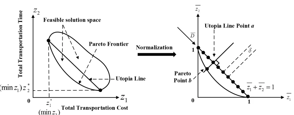
Contrary to the traditional solving approaches, such as weighted sum method that combines the different objectives linearly (Grosan & Abraham, 2010; Casetelletti, Pianosi & Restelli, 2013) or the lexicographic goal programming method that grants the objectives different priorities (Tamiz, Jones & Romero, 1998), Pareto optimality can provide the MTO and customers with an evenly distributed optimal solution set called “Pareto frontier” (Wang, Lai & Shi, 2011b). The MTO can select a suitable Pareto solution as the transportation scheme conveniently according to the Pareto frontier. Therefore, we aim to gain the Pareto frontier of the bi-objective optimization model. In this study, the Pareto frontier is gained by using the “normalized normal constraint method” (see in Figure 1) proposed by Messac, Ismail-Yahaya and Mattson (2003).
Figure 1. Normalized normal constraint method
In order to avoid the effect of the difference in the data scale and unit, the vector should be normalized by Equation (14).
(14)
After normalization, the two vectors and will be converted to (0, 1)T and
(1, 0)T. In the normalized two dimensional data space, the straight line linking (0, 1) and (1, 0) is
the “Utopia line”. The direction of the Utopia line is along which the Pareto points is distributed.
If the number of the Pareto solutions we prescribe is np, there exist np Pareto points and np
Utopia line points on the two lines. Each Utopia line point corresponds with a Pareto point, for example, the corresponding Pareto point of a i s b (see in Figure 1). Each Pareto point corresponds with a Pareto solution.
After setting the step between two adjacent Utopia line points, the coordinate of a Utopia line point can be gained by Equation (15).
(15) Where λ1u = u · δ and λ2u = 1 – u · δ for u{0, 1, ..., np – 1}. Obviously, the Utopia line points are
distributed evenly.
Finally, after adding Constraint (14) and the following Constraint (16) to the normalized single objective model with Formulas (2-12), the Pareto solution can be gained as shown in Figure 2.
(16)
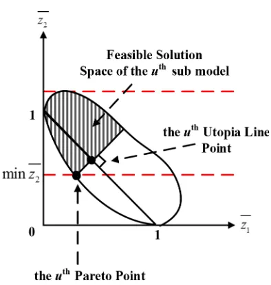
In the uth calculation, the Pareto point, Utopia line point and the feasible solution space of the
sub single objective model are shown in Figure 3 clearly.
Figure 3. Diagram of the uth step calculation
4. Experimental Case Study and Sensitivity Analysis
4.1. Determination of the Transportation Cost and Time
The respective average transportation speeds of the railway, highway and waterway are 60-70km/h, 80-90km/h and 20-30km/h. In this study, their speeds (unit: km/h) take the intermediate values as shown in Table 1.
Transportation Mode Speed
Railway 65
Highway 85
Waterway 25
Table 1. Container transportation speeds of the three transportation modes
The railway and highway container transportation cost on route is calculated by Equation (17).
(17) Where cm1 and cm2 are the unit transportation cost relevant to the volume of the consignment of
goods and the turnover of the consignment of goods, respectively.
The value of the transportation cost parameters of the two transportation modes are presented as shown in Table 2 according to the regulations proposed by the China Ministry of Railways and the China Ministry of Transport.
Mode Parameter Type of Container Unit
20ft 40ft
Highway cm1 15 12.5 CNY/TEU cm2 6 4.5 CNY/(TEU·km)
Railway cm1 449 305 CNY/TEU cm2 1.98 1.35 CNY/(TEU·km)
Table 2. Values of the transportation cost parameters
The waterway transportation cost is calculated by Equation (18).
(18) Where cW is the unit variable cost relevant to the volume of the consignment of goods. In the
inland waterway transportation of China, cW = 300 CNY/TEU.
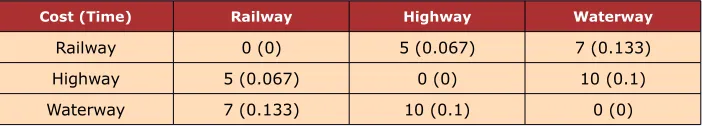
and can be calculated by using the average unit transshipping cost (unit: CNY/TEU) and time (unit: h/TEU) between the transportation modes that are shown in Table 3.
Cost (Time) Railway Highway Waterway
Railway 0 (0) 5 (0.067) 7 (0.133) Highway 5 (0.067) 0 (0) 10 (0.1) Waterway 7 (0.133) 10 (0.1) 0 (0)
4.2. Experimental Case Design
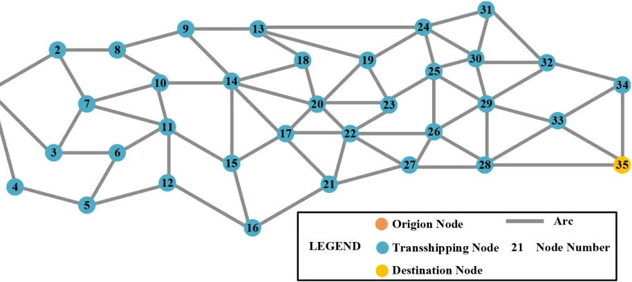
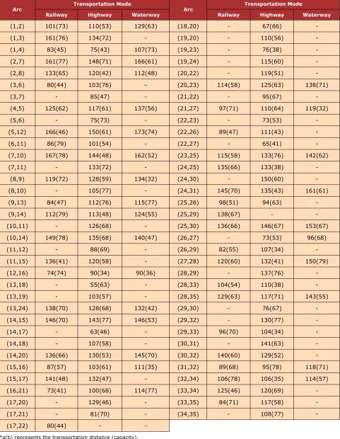
In this study, we design a 35-node multi-modal transportation network as shown in Figure 4. The topological structure of the multi-modal transportation network is modified from the study of Xiong and Wang (2014). The distances (unit: km) and capacities (unit: TEU) in the network are generated randomly according to the ranges based on real-world transportation and the corresponding transportation modes. The transportation distance and capacity of each arc in the multi-modal transportation network are presented in Table 4.
Arc Transportation Mode Arc Transportation Mode
Railway Highway Waterway Railway Highway Waterway
(1,2) 101(73) 110(53) 129(63) (18,20) - 67(66)
-(1,3) 161(76) 134(72) - (19,20) - 110(56)
-(1,4) 83(45) 75(43) 107(73) (19,23) - 76(38)
-(2,7) 161(77) 148(71) 166(61) (19,24) - 115(60)
-(2,8) 133(65) 120(42) 112(48) (20,22) - 119(51)
-(3,6) 80(44) 103(76) - (20,23) 114(58) 125(63) 138(71)
(3,7) - 85(47) - (21,22) - 95(67)
-(4,5) 125(62) 117(61) 137(56) (21,27) 97(71) 110(64) 119(32)
(5,6) - 75(73) - (22,23) - 73(53)
-(5,12) 166(46) 150(61) 173(74) (22,26) 89(47) 111(43)
-(6,11) 86(79) 101(54) - (22,27) - 65(41)
-(7,10) 167(78) 144(48) 162(52) (23,25) 115(58) 133(76) 142(62)
(7,11) - 133(72) - (24,25) 135(66) 133(38)
-(8,9) 119(72) 128(59) 134(32) (24,30) - 150(60)
-(8,10) - 105(77) - (24,31) 145(70) 135(43) 161(61)
(9,13) 84(47) 112(76) 115(77) (25,26) 98(51) 94(63)
-(9,14) 112(79) 113(48) 124(55) (25,29) 138(67) - -(10,11) - 126(68) - (25,30) 136(66) 146(67) 153(67)
(10,14) 149(78) 135(68) 140(47) (26,27) - 73(53) 96(68)
(11,12) - 88(69) - (26,29) 82(55) 107(34)
-(11,15) 136(41) 120(58) - (27,28) 120(60) 132(41) 150(79)
(12,16) 74(74) 90(34) 90(36) (28,29) - 137(76)
-(13,18) - 55(63) - (28,33) 104(54) 110(38)
-(13,19) - 103(57) - (28,35) 129(63) 117(71) 143(55)
(13,24) 138(70) 128(68) 132(42) (29,30) - 76(67)
-(14,15) 146(70) 143(77) 146(53) (29,32) - 130(77)
-(14,17) - 63(46) - (29,33) 96(70) 104(34) -(14,18) - 107(58) - (30,31) - 141(63)
-(14,20) 136(66) 130(53) 145(70) (30,32) 140(60) 129(52)
-(15,16) 87(57) 103(61) 111(35) (31,32) 89(68) 95(78) 118(71)
(15,17) 141(48) 132(47) - (32,34) 106(78) 106(35) 114(57)
(16,21) 73(41) 100(68) 114(77) (33,34) 125(46) 120(69)
-(17,20) - 129(46) - (33,35) 84(71) 117(58)
-(17,21) - 81(70) - (34,35) - 108(77)
-(17,22) 80(44) -
-*a(b) represents the transportation distance (capacity).
The transshipping capacity of each node in the multi-modal transportation network is shown in Table 5, where R, H and W represent the railway, the highway and the waterway, respectively.
Node R-H R-W H-W R-R H-H W-W
2 71 65 47 46 73 42
3 75 - - 66 59
-4 36 65 72 38 57 71
5 76 46 43 60 37 31
6 62 - - 43 73
-7 35 32 42 63 61 38
8 44 52 76 64 48 62
9 57 49 47 67 56 67
10 78 68 40 53 50 62
11 78 - - 34 34
-12 38 39 61 41 42 57
13 79 54 54 76 36 45
14 78 52 48 38 39 67
15 54 62 72 71 42 39
16 70 65 59 57 51 64
17 37 - - 80 32
-18 51 - - - 75
-19 - - - - 77
-20 70 63 68 35 55 69
21 78 38 68 78 54 34
22 63 - - 30 47
-23 32 55 58 69 75 69
24 72 78 34 71 48 54
25 77 47 33 73 36 52
26 64 59 57 34 69 52
27 68 41 69 50 49 45
28 67 68 77 43 42 55
29 50 - - 70 50
-30 63 55 58 52 35 71
31 39 65 53 76 37 70
32 65 75 31 39 77 62
33 32 - - 43 78
-34 71 57 38 60 59
4.3. Pareto Frontier of the Bi-objective Optimization Model
Then the case above is utilized to verify the feasibility of the proposed model and Pareto optimality. In this case, the transit period of goods is set to 60h (2.5 days). The containers carrying the consignment of goods are all 20ft ones and their number is 30 that is within the capacity of all the arcs and nodes. Then we will focus on the sensitivity analysis of the variation of the two factors by modifying them within a range. In the Pareto optimality, the number of Pareto solution is set to 13.
The bi-objective mixed integer linear programming model can be easily solved by mathematical programming software Lingo. Therefore, we use Lingo 11 to solve the bi objective optimization model based on Pareto optimality. The calculation of Lingo 11 is performed by a Lenovo Laptop with Intel Core i5 3235M 2.60GHz CPU and 4GB RAM. Its calculation results are shown in Table 6.
No. Pareto Solutions Times of LingoIteration
z1 (unit: CNY) z2 (unit: h)
1 72000 41.32 61
2 77250 40.92 822
3 93505 38.75 4384
4 100020 35.53 1156
5 107836 34.38 2254
6 114979 30.72 1634
7 123844 28.25 1845
8 125310 25.74 1566
9 136560 22.27 1496
10 146820 20.98 2037
11 151770 17.83 812
12 155575 14.41 804
13 163980 10.48 96
Table 6. Calculation results of Lingo 11
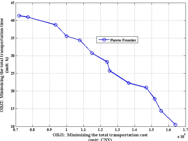
Figure 5. The Pareto frontier of the bi-objective optimization
The Pareto frontier in Figure 5 clearly indicates a compromised solution set on the two objectives of the bi-objective optimization model. The MTO can select one of the Pareto solutions as the transportation scheme conveniently based on the Pareto frontier, the MTO’s preference to which objective and the evaluation to the customer’s time satisfaction degree. For example, if the customer is satisfied that the total transportation time of the consignment of goods from its origin to the destination is within 20 to 25h, then the MTO can plan the transportation scheme by using the 9th Pareto solution.
4.4. Sensitivity Analysis of the Demand and Supply
The relationship between the demand and supply is the key point for the MTO to organize the multi-modal transportation and for the customer to select a MTO reasonably. Using the sensitivity analysis based on the Pareto frontier, the influence of the variation of the demand and supply can be clearly illustrated. In the following sensitivity analysis, NoC, TPoG and CoN are short for the number of containers, the transit period of goods and the capacity of the multi-modal transportation network, respectively.
4.4.1. Sensitivity Analysis of the Demand
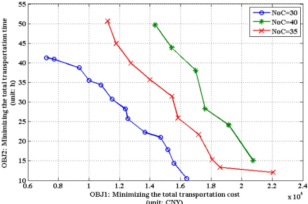
The demand of the customer contains two aspects, including the volume of a consignment of goods and the transit period of goods. First we analyze the influence of the variation of the goods volume on the Pareto frontier. Using NoC = 30 and TpoG = 60 as the primary data, we keep the TPoG constant and modify NoC from 30 to 35 and 40, and then gain a set of Pareto frontiers as shown in Figure 6.
Figure 6 indicates that with increase of the goods volume, the Pareto frontier moves from left to right. It is clearly that for the same transportation time, the transportation of goods with small volume can reduce the transportation cost. Similarly, for the same transportation cost, the transportation of goods with small volume can reduce the transportation cost. In addition, for a given multi-modal transportation network with limited available resource, the increase of the goods volume may exceed the capacity of part of its arcs and nodes, which will result in the decrease of the number of the Pareto solutions.
Based on Figure 6, the MTO can make a tradeoff between improving the transportation efficiency and reducing the transportation cost when serving the customers whose goods volume vary from each other. For example, if the MTO desires to extend the market and retain the customer, he can plan the transportation schemes base on the Pareto frontier on the right side and the evaluation to the customer’s time satisfaction degree. Because under the same time satisfaction degree, the Pareto frontier on the right side can provide the customer with large transportation capacity. However, the MTO must make a sacrifice on the transportation cost. Besides, the MTO can also plan the transportation schemes base on the figure above when the customers cannot determine their goods volume in advance.
Next we keep CoN constant (CoN = 30) and modify TPoG from 60 to 40 and 30, and gain a set of Pareto frontiers as shown in Figure 7.
Figure 7. Sensitivity analysis of the transit period of goods on the Pareto frontier
4.4.2. Sensitivity Analysis of the Supply
The capacity of the entire multi-modal transportation reflects the supply of the MTO. Using the CoN shown in Table 4 and Table 5 as the primary data, we keeping NoC and TPoG constant (NoC = 40, TpoG = 60), and modify the CoN by increasing 20% and 40%, and gain a set of Pareto frontiers shown in Figure 8.
Figure 8. Sensitivity analysis of the capacity of the multi-modal transportation network on the Pareto frontier
5. Conclusions
This study proposes a bi-objective optimization model to optimize the multi-modal transportation routing planning problem. Following contents are covered in it: (1) Minimizing the total transportation cost and total transportation time are set as the optimization objectives; (2) To balance the benefit between the two objectives, normalized normal constraint method is utilized to gain the Pareto frontier of the multi-modal transportation routing planning problem; (3) The influence of the variation of the demand and supply on the multi-modal transportation routing planning is gained by the Pareto frontier based sensitivity analysis; (4) The feasibility of the proposed model is verified and the sensitivity analysis is conducted by using a 35-node multi-modal transportation network to perform the numerical experiment.
The main contributions of this study are embodies in two aspects. First, we apply the normalized normal constraint method to gain the Pareto frontier of the bi-objective optimization for the multi-modal transportation routing planning problem. In this case, the multi-modal transportation routing planning scheme is a set that contains many candidate routes with different transportation cost and time, which can provide great flexibility for MTOs and customers to make decisions in this regard when considering various situations. Second, the Pareto frontier based sensitivity analysis is conducted, in which the influence of the variation of the demand and supply on the multi-modal transportation routing planning is gained. Through the sensitivity analysis, on one hand, MTOs and customers can better realize the dynamic multi-modal transportation market, on the other hand, the variation tendencies indicated by Figure 6 to Figure 8 can help MTOs and customers make decisions and modify strategies when planning the multi-modal transportation organization.
Acknowledgements
This study was supported by the National Natural Science Foundation Project (No.71390332-3) of the People’s Republic of China. The authors would also like to thank the editor of the journal and the anonymous reviewers, for their constructive suggestions and comments that lead to a significant improvement of this paper.
References
Atalay, S., Çanci, M., Kaya, G., Oguz, C., & Türkay, M. (2010). Intermodal transportation in Istanbul via Marmaray. IBM Journal of Research and Development, 54(6), 1-9.
http://dx.doi.org/10.1147/JRD.2010.2066090
Banomyong, R., & Beresford, A.K.C. (2001). Multimodal transport: the case of Laotian garment exporters. International Journal of Physical Distribution & Logistics Management,
31(9), 663-685. http://dx.doi.org/10.1108/09600030110408161
Bookbinder, J.H., & Fox, N.S. (1998). Intermodal routing of Canada-Mexico shipments under NAFTA. Transportation Research Part E: Logistics and Transportation Review, 34(4), 289-303.
http://dx.doi.org/10.1016/S1366-5545(98)00017-9
Caris, A., Macharis, C., & Janssens, G.K. (2008). Planning problems in intermodal freight transport: Accomplishments and prospects. Transportation Planning and Technology, 31(3), 277-302. http://dx.doi.org/10.1080/03081060802086397
Casetelletti, A., Pianosi, F., & Restelli, M. (2013). A multi-objective reinforcement learning approach to water resources systems operation: Pareto frontier approximation in a single run.
Water Resources Research, 49(6), 3476-3486. http://dx.doi.org/10.1002/wrcr.20295
Fan, Z.Q., & Le, M.L. (2011). Research on multimodal transport routing problem with soft time windows under stochastic environment. Industrial Engineering and Management, 16(5), 68-72. http://dx.doi.org/10.3969/j.issn.1007-5429.2011.05.011
Fu, X.F. (2013). Study of system on management of logistics safety and decision-making of emergency response at multimodal transport, Doctoral Thesis, Chang’an University, Xi’an, China. http://dx.doi.org/10.7666/d.D559273
Grosan, C., & Abraham, A. (2010). Approximating Pareto frontier using a hybrid line search approach. Information Sciences, 180(4), 2674-2695. http://dx.doi.org/10.1016/j.ins.2009.12.018
Janic, M. (2007). Modelling the full costs of an intermodal and road freight transport network.
Transportation Research Part D: Transport and Environment, 12(1), 33-44.
Jiang, J., & Lu, J. (2008). Research on optimum combination of transportation modes in the container multimodal transportation system. Proceedings of the 8th International Conference of Chinese Logistics and Transportation Professionals-Logistics: The Emerging Frontiers of
Transportation and Development in China. Chengdu, China. July 31-August 3.
http://dx.doi.org/10.1061/40996(330)99
Liu, J., He, S.W., Song, R., & Li, H.D. (2011). Study on optimization of dynamic paths of intermodal transportation network based on alternative set of transport modes. Journal of the
China Railway Society, 33(10), 1-6. http://dx.doi.org/10.3969/j.issn.1001-8360.2011.10.001
Messac A., Ismail-Yahaya, A., & Mattson, C.A. (2003). The normalized normal constraint method for generating the Pareto frontier. Structural and Multidisciplinary Optimization, 25(2), 86-98. http://dx.doi.org/10.1007/s00158-002-0276-1
Sun, B., & Chen, Q.S. (2013). The routing optimization for multi-modal transport with carbon emission consideration under uncertainty. Proceedings of the 32nd Chinese Control
Conference. Xi’an, China. July 26-28.
http://ieeexplore.ieee.org/stamp/stamp.jsp?tp=&arnumber=6640875
Sun, Y., Lang, M.X., & Wang, D.Z. (2015). Optimization Models and Solution Algorithms for Freight Routing Planning Problem in the Multi-modal Transportation Networks: A Review of the State-of-the-Art. The Open Civil Engineering Journal, 9, 714-723.
http://dx.doi.org/10.2174/1874149501509010714
Tamiz, M., Jones, D., & Romero, C. (1998). Goal programming for decision making: An overview of the current state-of-the-art. European Journal of Operational Research, 111(3), 569-581. http://dx.doi.org/10.1016/S0377-2217(97)00317-2
Wang, B., & Wang, X.L. (2013). Genetic algorithm application for multimodal transportation networks. Information Technology Journal, 12(6), 1263-1267.
http://dx.doi.org/10.3923/itj.2013.1263.1267
Wang, F., Lai, X.F., & Shi, N. (2011b). A multi-objective optimization for green supply chain network design. Decision Support Systems, 51(2), 262-269.
http://dx.doi.org/10.1016/j.dss.2010.11.020
Wang, Q.B., & Han, Z.X. (2010). The optimal routes and modes selection in container multimodal transportation networks. Proceedings of 2010 International Conference on
Optoelectronics and Image Processing, Haikou, China, November 11-12.
http://dx.doi.org/10.1109/ICOIP.2010.276
Wang, X., Chi, Z.B., & Ge, X.L. (2011a). Research and analysis for time-limited multimodal transport model of vehicle. Application Research of Computers, 28(2), 563-565.
http://dx.doi.org/10.3969/j.issn.1001-3695.2011.02.044
Winebrake, J.J., Corbett, J.J., Falzarano, A., Hawker, J.S., Korfmacher, K., Ketha, S. et al. (2008). Assessing energy, environmental, and economic tradeoffs in intermodal freight transportation. Journal of the Air and Waste Management Association, 58(8), 1004-1013.
http://dx.doi.org/10.3155/1047-3289.58.8.1004
Xiong, G.W., & Wang, Y. (2014). Best routes selection in multimodal networks using multi-objective genetic algorithm. Journal of Combinatorial Optimization, 28(3), 655-673.
http://dx.doi.org/10.1007/s10878-012-9574-8
Yang, X. (2013). Research on the optimal routes and modes selection in container multimodal
transportation networks consider of the transshipment time. Master Thesis. Dalian Maritime
University, Dalian, China. http://d.g.wanfangdata.com.cn/Thesis_Y2300921.aspx
Zhang, J.Y., & Guo, Y.H. (2002). A multimode transportation network assignment model.
Journal of the China Railway Society, 24(4), 46-50.
http://dx.doi.org/10.3321/j.issn:1001-8360.2002.04.024
Zhang, Y.H., Lin, B.L., Liang, D., & Gao, H.Y. (2006). Research on a generalized shortest path method of optimizing intermodal transportation problems. Journal of the China Railway
Society, 28(4), 22-26. http://dx.doi.org/10.3321/j.issn:1001-8360.2006.04.005
Journal of Industrial Engineering and Management, 2015 (www.jiem.org)
Article's contents are provided on a Attribution-Non Commercial 3.0 Creative commons license. Readers are allowed to copy, distribute and communicate article's contents, provided the author's and Journal of Industrial Engineering and Management's names are included.