AFRICAN BUFFALO OPTIMIZATION AND THE RANDOM IZED INSERTION ALGORITHM FOR THE ASYMMETRIC TRAVELLING SALESMANS PROBLEMS

(1)

ISSN: 1992-8645 www.jatit.org E-ISSN: 1817-3195

A NOVEL RANK BASED CO-LOCATION PATTERN MINING

APPROACH USING MAP-REDUCE

1

M.SHESHIKALA, 2 D. RAJESWARA RAO, 3 R.VIJAYA PRAKASH

1

Research Scholar ., Department of Computer Science and Engineering , KL University, Vadeshwaram,

Guntur, India

2

Professor., Department of Computer Science and Engineering , KL University, Vadeshwaram, Guntur,

India

3

Professor., Department of Computer Science and Engineering , SR Engineering College, Warangal, India

E-mail: [email protected], [email protected], [email protected]

ABSTRACT

With the increase in spatial data analysis, the co-location patterns and its dependencies are used to discover the complex patterns on spatial databases. Most of the traditional spatial data mining techniques have been implemented based on the assumption that the data is meaningful and clean. It is essential to study the data integration issues along with spatial co-locating patterns. Generally, spatial co-location mining algorithms are used to discover the spatial objects and its dependencies among them. As the data size increases, the co-location objects and its patterns are difficult to process on complex spatial objects. In this paper, an optimized spatial co-locating pattern mining framework was developed to discover the highly ranked correlated patterns using the hadoop framework. This MapReduce model was used to minimize computational time and space on complex spatial databases. Finally, the experimental results on the complex spatial data are evaluated using the proposed framework and the traditional hadoop based pattern mining models

.

Keywords: Spatial Dataset, Co-Location Models, Association Rules, Prevalence Threshold, Mapreduce.

1. INTRODUCTION

Large amounts of spatial data collected through real time geographical information system, remote sensing and other applications, make it essential to design and develop tools for the interesting patterns from large spatial datasets. Most of the spatial mining models use spatial objects with the known geographic location. There exist different sources of spatial information to be uncertain, inconsistence, incompleteness, imprecision and error.

Data preprocessing is a process to improve the quality of the spatial data objects through spatial data mining techniques. It includes, the understanding of spatial metadata and its relationships, checking constraints in spatial objects, eliminating noisy data, removing duplicate objects and filtering inconsistent data objects. So, data preprocessing is not a simple task to filter the noisy and inconsistent spatial objects into the cleaned objects. These make it difficult to use the

traditional tools to manipulate and manage. About 85% of data is associated with the spatial position.

(2)

[image:2.612.108.289.74.416.2]

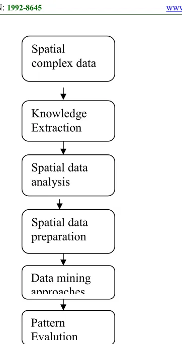
Figure 1: Basic Spatial Data Mining Framework

In the first phase, complex spatial objects from different sources are extracted to form a complex data set. This complex data has a large number of instances with structured, semi-structured and unstructured information. This complex data has incomplete, noisy and inconsistent data for knowledge extraction in different domain applications such as remote sensing, wireless networks, medical, etc. In the third phase, spatial objects and its statistical relationships are analyzed for data preprocessing [3][4]. In the data preprocessing phase, noisy and inconsistent data were filtered to refine the spatial objects based on domain knowledge and data analysis. In the data mining phase, different parallel and incremental approaches are performed on the large complex data for pattern evaluation. Extracting patterns or rules from the spatial objects are more difficult than the identifying correlated rules in traditional categorical and continuous objects due to the noise and uncertainty among them. In the final phase, i.e. pattern evaluation, patterns are analyzed and validated using statistical measures.

1.1 Spatial Association Miner

In data mining, spatial association mining is one of the most commonly used approaches for data analysis in different fields. It is applicable to different data types, such as ration-scaled, continuous, spatial, multimedia arts. Spatial association rule mining can be stated as the extraction of co-related rules, spatial associations or implicit rules stored in spatial datasets usually; spatial association rules are generated from a complex dataset on the basis of frequent or infrequent patterns. Spatial association rules mainly categorized into three types based on spatial association among the features of the same objects in the same spatial patterns and spatial association among different objects in the different spatial patterns. The first type is known as spatial length wise patterns. Second and third types are known as spatial traversal relations [5].

1.2 Spatial Co-located Patterns

Spatial data analysis is an essential part in spatial machine mining field with a large number of real-time applications. Examples include: co-locating human species discovery, co-co-locating hotels discovery, co-located services in mobile phones, etc. Along with spatial attributes, the non-spatial attributes and its metadata also help to improve the lo-located mining results. Traditional co-location models fail to use non-spatial elements in spatial data, which leads to inconsistent results. Also, most of the models consider similarity distance as a metric to decide the closest relationship between the spatial features. As it is difficult to initiate the prevalence metric for each spatial data without any prior knowledge.

A frequent spatial co-located pattern extracts the spatial rules whose objects frequently occurred together. Example, in some cities, colleges and parks often occurred together and they are treated as frequent co-located pattern of the city. There are several techniques have been introduced in the literature to improve the co-location patterns. The literature works can be categorized into three kinds: the join based methods, the partial join methods and the join less models. The join based method is similar to the Apriori method with large number of database scans and needs to spend a lot of time and memory for pattern joining operation. In the partial join method, entire spatial objects partitioned into two parts, i.e. one is inter and the other is intra, but it is very complex to divide the spatial objects into real-time objects. Although, join less doesn’t need

Spatial

complex data

Knowledge

Extraction

Spatial data

analysis

Spatial data

preparation

Data mining

approaches

(3)

to perform patterns join operation, it may use complex data structures on specific conditions [6].

1.3 Spatial Co-location Instance (SCI)

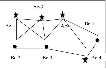
SCI can be defined as the set of spatial objects whose events have closest relationships with each other. The closest relationship represents the correlation between the spatial elements that are identified within the specified threshold.

[image:3.612.89.302.295.435.2]

For example: the set { Ae-1,Ae-3,Be-2,Be-3} is a spatial co-location instance because all of its objects have closest neighborhood relationship with each other as shown in Fig 2.

Figure 2.Spatial Relationships

MapReduce is a programming environment for generating high dimensional datasets and process them efficiently. Each spatial developer has to define their own mapper-reducer operations on complex datasets. In the Mapper interface, each input data is taken as input to produce a set of intermediate (key, value) pairs. In the reducer interface, all intermediate (key, value) pairs are merged using the, same key. Big data is complex dataset that has the following main features [7] [8]:

• Volume

• Variety

• Velocity

• And Veracity.

Hadoop is an open source framework with high scalability, low cost, high efficiency, good portability and reliability. These features have proven hadoop is one of the best solutions to distributed computing for large scale data. Programs written in the standard programming style are automatically parallelized and executed on a specified number of cluster nodes. Hadoop framework will take care of the internal details of

the input data partitioning, scheduling across the cluster nodes and machine failures.

1.4 Limitations and scope in Hadoop based Co-location Mining

• Generates a large number of patterns with a small change in prevalence threshold.

• Co-location patterns suffer with spatial outliers in the grid space.

• Memory and time complexity increases as the number of features increases.

In the Section II, related work of the parallel spatial co-location mining approaches and its limitations are discussed. In section III, we have discussed the Hadoop [11] [12] based spatial pattern miner on complex data and its performance are evaluated on the different data sizes...finally, Section IV describes about conclusion and future scope.

2. RELATED WORK

2.1 Threshold based Spatial Miners

Lee et al. [5] proposed a model to extract highly correlated patterns in a set of transactions using the threshold based distance measure. Let

1 2 n

I

=

{ ins ,ins ,....,ins }

be the set of values in the transaction and DB denotes the set of transactions. Each transaction

τ

has a set of elements such that

τ

∈

I

. Let

P

∈

I

be the set of correlated elements referred as a pattern. A pattern with m-elements is an m-pattern.

Let, support of the pattern is denoted as, which represents the number of transactions satisfying the pattern

P

in DB. The pattern

P

is said to frequent in the spatial objects, if it satisfies the minimum support measure as

S( P )

≥

minsup

---Eq.1 Where min-sup is the user defined minimum support value. The all-confidence computation on the pattern

P

is computed as the ration of support value to the maximum support of an element in the set itself.

i i

all conf ( P) S(P) / (Max(p )| p

−

=

∈

P)

……Eq.2 Finally, the pattern

P

is said to be correlated pattern if it satisfies two conditions as

S( P )

≥

minsup

And

all

−

conf ( P )

≥

min allconf

Where

min allconf

the user is defined minimum confidence.

Ae-1

Ae-3

Ae-Be-2 Be-3 Ae-4

(4)

[image:4.612.89.303.163.358.2]

Table 1:_{Spatial Database}

TID Spatial Object

T-1 (100.200),(102,150),(200,120)

T-2 (123,235),(250,500)

T-3 (100,450),(250,350)

T-4 (102,150),(100.200),(129,340)

T-5 (200,120),(250,350),(123,235)

T-6 (250,350),(100,450)

T-7 (100.200),(100,450),(102,150)

T-8 (100,450),(250,500)

T-9 (102,150),(123,235)

T-10 (100.200),(200,150)

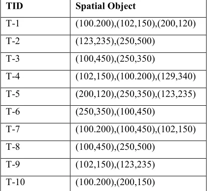
Example 1: The spatial database is shown in Table

1 have 10 transactions. The set of spatial objects is {(100,200), (102,150), (200,120), (123,235), (250,500), (100,450), (250,350), (200,150), (250,500), and (129,340)}. The set of elements {(100,200), (102,150)} is said to be a 2-pattern.This pattern occurs in 3 transactions {1, 4, T-7}.Therefore the support of the given pattern is

S(P)

=3.

If the user defined minimum support is 1.5 then {(100,200), (102,150)} is a frequent pattern because

S( P )

≥

minsup

. S ((100,200)) =4 and S ((102,150)) =4.

all

−

conf ( P )

=3/Max{4,4}=3/4=0.75.

If the user specified all-conf value is 0.61, then the given pattern objects are correlated to each other because

all

−

conf ( P )

≥

min allconf

.

The author [6] has implemented h-confidence measure to discover hyper clique correlated patterns. These patterns are set of objects with common behavior and strongly correlated to each other. The main issue in the h-confidence property is a rare item problem.

Haung’s[7] implemented a model to find the maximal clique correlated objects in the dataset.

This model doesn’t use membership ratio for the cliques, this violates the maximal clique definition and common relationship. Assume clique-A has three elements {A-5, A-10, A12} and clique-2 has {A-14, A-12, A19}, element {A-12} is a common element between the two cliques. Extracting useful and rare spatial patterns from complex objects is very difficult than finding the relevant patterns from conventional continuous and nominal data types due to its variation of spatial relationships and locations. The major issue in mining co-location rules and patterns from complex spatial objects can be summarized as follows:

Co-location Mining approach:

Given Input:

• Spatial-Mining framework SF

• A set of n-Boolean spatial-features and its types as

BSO

=

{bf ,bf ,....,bf }

₁ ₂ _n

• A set of k records, each record has <inst-id, spat-feature type, location>where spatial features belongs to BSO.

• Find neighborhood relations in data objects.

• User defined thresholds. Find:

• The conditional probability p indicates the occurrence of spatial objects in A, the prediction of occurrences of B in a nearby distance is p. Co-location patterns with high probabilistic conditional value.

Procedure:

Initialize the one-set co-located set with the given spatial data.

Construct 2-set co-location patterns using join- prune strategy using the 1-set items.

For each set 2…n-1 does

Generate the candidate sets on the co-located patterns using traditional apriori approach.

Construct spatial instances table and prune the table based on nearest neighborhood.

Filter the rules based on co-locations patterns.

Generate co-locations rules from patterns.

(5)

In the above traditional co-location patterns, a large number of candidate sets for each spatial feature are generated. This approach takes more memory and time for pattern and rule generation process. This approach fails to generate dynamic patterns in real-time spatial objects with varying locations.

[8] Soung , proposed a co-location pattern extraction using density based approach. They divided spatial objects into partitions and extracting spatial features in high dense regions first. This model reduces the join operation [13] [14] on the spatial features. The basic pattern evaluation process with the pre-defined set of partitions and sizes is formulated below:

2.2 Grid Density based Pattern Miner

Input:

Spatial data objects and features

Output:

Co-location patterns or rules

Parameters:

C:co-location size

CSc:c size candidate sets

Lc:c size patterns

Procedure:

Construct the grid over the spatial objects space

Randomly assign hashed objects into partitions

L1:1-set spatial object set and c=1

While Lc!=null do

Generate CSc+1 candidate sets

Identify Lc+1 patterns based on density in the grid

c=c+1;

done

Return union of all patterns.

Generally, most of the traditional techniques adopt the 3-step process ,which (a) firstly it builds the nearest spatial neighborhood relationships using the predefined threshold.(b) secondly, collects the candidate locations objects.(c) finds the co-location patterns on the candidate co-co-locations. The threshold based technique requires the users to specify the minimum threshold in advance for co-location patterns. However, it is not easy to select the predefined threshold to each spatial data due to the following issues:

1) A small change in prevalence threshold may generate a large number of patterns.

2) A small value of the distance threshold may result many clique spatial objects of prevalent co-locations.

3

.

HADOOP BASED CO-LOCATION

PATTERN MINER

For the given spatial database, a nearest neighbor relationship [15] [16] and minimum prevalence threshold are computed in two main steps:

1. Spatial neighborhood grid partition 2. Hadoop based co-location event patterns

search.

In the first case, the entire data objects are partitioned over the co-location search space and in the second case, co-location spatial objects are searched in the Map phase synchronously, and then merged in the Reducer phase to find the prevalent co-located event sets[9][10].

Conditional Neighborhood: Let G(V,E) be a spatial neighbor graph with Vertex set V and Edge set E,

N( v∈V ) is the set of star neighborhood relationships of vertex “v” adjacent to “u” including “v” itself, which satisfies the given constraint as

∀x , ye e∈V : ( x , y )e e ∈E

<

e e

and

x .type y .type

Example for Spatial Neighborhood Relationship:

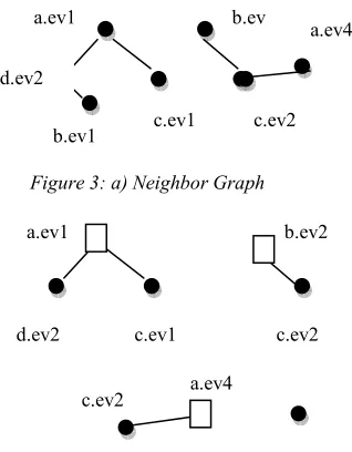
Figure 3: a) Neighbor Graph

Figure 3: b) Edge partitioning graph

In the above Figure 3, a) describes the spatial nearest neighbor relationships of the given sample

a.ev1

d.ev2

b.ev1 c.ev1 b.ev

c.ev2 a.ev4

a.ev1

d.ev2 c.ev1

b.ev2

a.ev4 c.ev2

[image:5.612.351.510.496.700.2]

(6)

of spatial objects. Here a, b, c, d represents the set of event type and numerical number represents the object. <a.ev1, d.ev2, b.ev1, c.ev1> and <b.ev2, c.ev2, a.ev4> represent neighbor graphs along with relations.

………

……

[image:6.612.313.524.129.261.2]

……

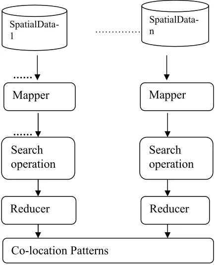
Figure 4: Hadoop based Co-location Architecture

Figure b) represents the edge partitioning graph using conditional neighborhood relationship. The general framework of MapReduce based co-locating pattern mining is shown in the Figure 4. The Map-Reduce hadoop framework splits the input spatial objects into separate blocks in order to represent each object in grid space. Using the geo-location and space partitioning method, a grid identification number is allotted to each spatial data object. In the Map operation, each key-value pair has grid number and its object value in the form of <key, value>. After Mapper phase, Reducer function initializes the given threshold as ‘dist’ and computes all the nearest neighbor elements in the key value pairs and outputs another intermediate key value pair <key,, value’>.

3.1 Relationship between Master and Slave Nodes

The Master (Name Node) manages the file system namespace operations like opening, closing, and renaming files and directories and determines the mapping of blocks to Data Nodes along with

regulating access to files by clients. Master {Job tracker} is the point of interaction between users and the map/reduce framework.

Figure 5: Relationship between Master and Slave Nodes

When a map/reduce job is submitted, Job tracker puts it in a queue of pending jobs and executes them on a first-come/first-served basis and then manages the assignment of map and reduce tasks to the task trackers.

Slaves (Data Nodes) are responsible for serving read and write requests from the file system’s clients along with perform block creation, deletion, and replication upon instruction from the Master (Name Node). Slaves {task tracker} execute tasks upon instruction from the Master {Job tracker} and also handle data motion between the map and reduce phases.

Mapper Procedure

Spatial objects (Key k,Value Oi) For each object ob∈O_i

Do

Check the prevalent type If exists

i

O=Oi-ob; End if End for m=pattern size;

check the cliqueness in the m size candidate sets. For each instance in candidate sets

If cliqueness exist emit(event-set,object); end if

done

End procedure

Reducer Procedure

Reducer(Key=event-set,value)

SpatialData-1

SpatialData-n

Mapper

Search

operation

Reducer

Co-location Patterns

Mapper

Search

operation

[image:6.612.77.294.162.429.2]

(7)

ISSN: 1992-8645 www.jatit.org E-ISSN: 1817-3195 load('threshold');

λ=

Pi=computePI(value); If(Pi>=λ)

Then

Emit(event-set,Pi);

1

ϕ

=generate_singlepatterns(patterns,event-set)

2

ϕ

= generate_twocandidatesets(patterns,event-set)

For each rule in

ϕ

₁

For each rule in

ϕ

₂ do

1 2

( ,

)

corr

r

σ

=

RankedCorr

ϕ ϕ

if

r

σ

_corr≥

min thres

then

if lift(

ϕ ϕ

1

,

2) ≥

conf

min

then FPatt ← FPatt ∪_{

1

,

2

ϕ ϕ

}

else if lift(

ϕ ϕ

₁

,

₂) ≥

conf

_minand sup(

¬

ϕ

₁

,

¬

ϕ

₂ )

≥

ρ

_min then

IPatt ← IPatt ∪_{

1

,

2

ϕ

¬

}

endif

if

r

σ

_corr

≤

-

min thres

then

if lift(

ϕ

₁

,

¬

ϕ

_k) ≥

conf

_min then

1

,

k

ϕ

¬

ϕ

} endif

if lift(

¬

ϕ ϕ

₁

,

_k) ≥

conf

_min then

1

,

k

ϕ ϕ

¬

}

endif endif

Save(event-set,object); End if

Lift calculates the ratio between the rules support and confidence of the item set in the rule consequent based on the each selected class.

: Probability of occurrence of an item in samples of ith class.

pr

(itm , )

i

D

: Probability of occurrence of an

item in a dataset of ith class.

Correlation(

φ

₁,

φ

₂)=

1 2 2 1

2 2

1 2 2 1

| D | lift(i/ i

,

) | D | lift(i

, )

| D | lift(i/ i

,

)

lift(i/ i

, )

φ φ

∈

−

∈

−

∈

i j

1 2 1 2

1 2

φ φ φ φ

φ φ

= Correlation

Corr ( , )

Ranke ( ,

( x ) /

d )

prob( ( y ))

Complexity of the algorithm:

Time complexity: M*log(n); Where M is the number of data nodes//slaves; and n is the data size.

4. EXPERIMENTAL COMPARISON ON

SPATIAL DATABASE

[image:7.612.311.548.441.552.2]

In this experimental study, we have used synthetic spatial data sets with different event types such as 30, 50. The user defined neighbor distance is 10. We used 3 cluster nodes, one is master and two are slaves. We have implemented these models on Amazon cloud services with Linux as operating system. Also, the apache hadoop framework was used for co-location pattern miner. We have analyzed the co-location patterns with different minimum prevalence threshold.

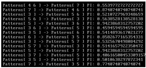
Figure 6: Pattern Evaluation With PI Measure.

(itm /

_i _i

) /

(itm ,

_i

)

lift

=

pr

D

pr

D

(itm /

_i _i

)

(8)

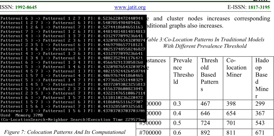
[image:8.612.91.528.70.288.2]

Figure 7: Colocation Patterns And Its Computational Measures

Table 2: Conditional Graphs With Varying Distance Threshold And Size

#Instance ssize

#Clust er nodes

Distanc e Thresho ld

Conditional Neighbors graphs

#100000 2 10 58

#200000 3 15 119

#500000 4 15 263

#700000 5 15 410

Table 2, describes the instances-set size of grid space and different cluster nodes in hadoop environment with varying distance threshold. As the size of input size and cluster nodes increases corresponding conditional graphs also increases.

Figure 8: Conditional Graphs With Varying Distance Threshold And Size

Fig 8, describes the instances-set size of grid space and different cluster nodes in Hadoop environment with varying distance threshold. As the size of input

size and cluster nodes increases corresponding conditional graphs also increases.

Table 3:Co-Location Patterns In Traditional Models With Different Prevalence Threshold

#Instances size

Prevale nce Thresho ld

Thresh old Based Pattern s

Co-location Miner

Hado op Base d Mine r

#100000 0.3 467 398 299

#200000 0.4 646 654 367

#500000 0.5 724 701 543

#700000 0.6 892 811 671

Table 3, describes the different prevalence threshold and its corresponding co-location patterns in different traditional models i.e., Threshold based model, Co-location pattern miner and hadoop based model.

Figure 9: Co-Location Patterns In Traditional Models With Different Prevalence Threshold.

Fig 9, describes the different prevalence threshold and its corresponding co-location patterns in different traditional models i.e., threshold based model, Co-location pattern miner and Hadoop based model.

5. CONCLUSION

[image:8.612.85.300.330.449.2] [image:8.612.309.522.359.485.2] [image:8.612.91.300.530.651.2]

(9)

hadoop based pattern mining models. In the future work, we will minimize the co-location patterns along with mapper and reducer execution time using a new data structure

.

REFERENCES

[1] Li, Dapeng; Sander, Joerg; Nascimento, Mario A.; Kwon, Dae-Won,"Discovering Spatial Co-Clustering Patterns in Traffic Collision Data",Association for Computing Machinery — Nov 5, 2013.

[2] Yue Jiang, Yue Jiang; Lizhen Wang, Lizhen Wang; Ye Lu, Ye Lu; Hongmei Chen, Hongmei Chen"Discovering both positive and negative co-location rules from spatial data sets",Institute of Electrical and Electronics Engineers — Jan 23, 2010.

[3] Morimoto, Yasuhiko,"Co-location pattern mining for unevenly distributed data:

algorithm, experiments and

applications",International Journal of Computational Science and Engineering , Volume 5 (3) – Jan 1, 2010.

[4] Dai, Bi-Ru; Lin, Meng-Yan,"Efficiently Mining Dynamic Zonal Co-location Patterns Based on Maximal Co-locations",Institute of Electrical and Electronics Engineers — Jan 20, 2012.

[5] Venkatesan, M.; Thangavelu, Arunkumar,"A multiple window–based co–location pattern mining approach for various types of spatial data",International Journal of Computer Applications in Technology , Volume 48 (2) – Jan 1, 2013.

[6] Canh, Tran Van; Gertz, Michael,"A Constraint Neighborhood Based Approach for Co-location Pattern Mining",Institute of Electrical and Electronics Engineers — Aug 17, 2012. [7] Yan, Huang; Jian, Pei; Hui, Xiong,"Mining

Co-Location Patterns with Rare Events from Spatial Data Sets",Geoinformatica , Volume 10 (3) – Sep 1, 2006.

[8] Yoo, Jin Soung; Boulware, Douglas; Kimmey, David,"A Parallel Spatial Co-location Mining Algorithm Based on MapReduce",Institute of Electrical and Electronics Engineers — Jun 27, 2014.

[9] You Wan, You Wan; Jiaogen Zhou, Jiaogen Zhou; Fuling Bian, Fuling Bian,"CODEM: A Novel Spatial Co-location and De-location Patterns Mining Algorithm",Institute of Electrical and Electronics Engineers — Jan 18, 2008.

[10] Feng Qian, Feng Qian; Liang Yin, Liang Yin; Qinming He, Qinming He; Jiangfeng He, Jiangfeng He,"Mining spatio-temporal co-location patterns with weighted sliding window",Institute of Electrical and Electronics Engineers — Jan 20, 2009.

[11]Rashmi Agrawal ,“Design and Development of Data Classification Methodology for Uncertain Data “,Indian Journal of Science and Technology,2016 Jan, 9(3),pp. 1-12

[12] K. Anuradha, N. Sairam ,“Spatio-temporal Based Approaches for Human Action Recognition in Static and Dynamic Background: a Survey “,Indian Journal of Science and Technology,2016 Feb, 9(5), pp.1-12.

[13] M. Y. Lin, P. Y. Lee, and S. C. Hsueh, “Apriori-based Frequent Itemset Mining Algorithms on MapReduce,” in Proceedings of the International Conference on Ubiquitous

Information Management and

Communication, 2012, pp. 1–8.

[14] N. Li, L. Zeng, W. He, and Z. Shi, “Parallel Implementation of Apriori Algorithm based on MapReduce,” in Proceedings of ACIS International Conference on Software Engineering”,Artificial Intelligence, Networking and Parallel/Distributed Computing, 2012, pp. 236–241

[15] R. Agrawal and J. Shafer, “Parallel Mining of Association Rules,” IEEE Transactions on Knowledge and Data Engineering, 1996, pp. 962–969.