ASSOCIATION RULE MINING BASED VIDEO CLASSIFIER WITH LATE ACCEPTANCE HILL CLIMBING APPROACH

AN ARTIFICIAL BEE COLONY ALGORITHM WITH

MODIFIED SEARCH STRATEGIES FOR GLOBAL

NUMERICAL OPTIMIZATION

1_{JIANFENG QIU,} 2_{JIWEN WANG,} 3_{DAN YANG,} 4_{JUAN XIE}

1, 2, 3

School of Computer Science and Technology, Anhui University, Hefei 230039, Anhui, China

4_{Department of Mathematics & Physics，Anhui University of Architecture, Hefei 230022, Anhui, China}

ABSTRACT

The Artificial Bee Colony (ABC) algorithm based on swarm intelligence is a more competitive algorithm than other Evolution Algorithm (EA). The results of recent studies indicate that the ABC algorithm has many advantages but it has two major weaknesses: one is slower convergence speed; the other is getting trapped in local optimal value early. Inspired by differential evolution (DE), different with other improved ABC algorithm based Differential Evolution (DE), we propose a modified ABC algorithm, named it ABC/current-to-best/1, by introducing the best food source (the best solution) and randomly choosing food source (the random solution). Experiments are conducted on a group of 24 benchmark functions. The results testify the performance of ABC/current-to-best/1 algorithm better than original ABC and some pre-existing improved ABC algorithm.

Keywords: Artificial Bee Colony, Global Numerical Optimization, Search Strategy, Differential Evolution

1. INTRODUCTION

Population-based algorithm can be mainly classif ied into two types: Evolutionary Algorithm (EA) an d Swarm Intelligence Algorithm (SIA). The two po pulation-based algorithms have a common feature: all possible solutions in population can be moved to ward the optimized solution by applying some oper ators based on the fitness value. In EA, The popular algorithms include Genetic Algorithm(GA)[1],Gen etic Programming(GP)[2],Evolution Strategy(ES)[3 ] and Evolution Programming(EP)[4]. Since the late 1990s, Differential Evolution (DE) has emerged as a competitive EA algorithm [5-6]. From then on, D E has been applied in tackling multimodal, multiobj ective, constrained and dynamic optimization probl ems extensively and has got better experimental res ults than other EAs. As for swarm intelligence-base d algorithm, Bonabeau has defined the swarm intell igence as “...any attempt to design algorithms or dis tributed problem-solving devices inspired by the co llective behavior of social insect colonies and other animal societies...” [7].The classical examples of s warm intelligence algorithms include Ant Colony O ptimization(ACO) algorithm which simulates foragi ng behavior of ants[9], Particle Swarm Optimizatio n (PSO) algorithm which is composed of birds and simulates the social behavior of bird flocking[9], Vi rtual bee algorithm(VBA)[10],Artificial bee colony (ABC) algorithm[11] and so on. Moreover some hy

brid methods based EA and SIA have been propose d to compensate some drawbacks in using EA or SI A alone [12-15].

In order to balance exploration and exploitation well, inspired by DE [4], we propose a new modifie d searching strategy which is not only improving ex ploitation but also avoiding getting trapped into loc al optimization early.

The rest of this paper is organized as follows. In section 2, we outline classical ABC algorithm and s ome important variants of ABC algorithm. Section 3 proposes modified ABC algorithm, explaining im proved searching strategies in detail. The experime ntal parameters settings and results are described in section 4. Section 5 concludes this paper with a disc ussion.

2. CLASSICAL ABC ALGORITHM AND

IMPORTANT VARIANTS

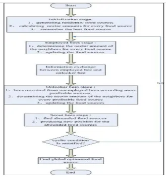
[image:2.612.145.480.238.597.2]

Artificial Bee Colony(ABC) algorithm introduce d by karaboga was first used to find an optimal solu tion in numerical optimization by simulating the be havior of foraging selection[11].The collective intel ligence in ABC is composed of three components: f ood sources, employed bees, unemployed bees(onlo oker bees, scout bees) and two behavior models: re cruitment and abandonment. The whole algorithm s tructure is described as follows:

Figure 1: Flowchart Of The Classical ABC Algorithm

In reference [11], a detailed explanation was mad e for classical ABC algorithm. In this section, we o utline the major idea of the algorithm. As we can se e from Figure 1, three major stages are included int o ABC algorithm, employed bees stages, onlooker bees stages and scout bees stages respectively.

2.1 Initialization Stage

In ABC algorithm, every food source position

,1 ,2 ,

( , ... )

i i i i D

X = x x x _{, where D is the number of problem}

dimension, representing a possible solution. The ini tial population should contain the range as much as possible by uniformly randomizing individuals with in the search space. This operation is defined as in [16]:

min (0,1)( max min)

j j j j

i

x =x +rand x −x (1)

Where,

x

_ijis the jth component of the ith food so

pectively. In ABC algorithm, the amount of nect ar in a food source represents the quality of the solution. In practice, the amount of nectar can b e expressed with the optimal value of the objecti ve function. So, the final step in initialization sta ge is to calculate the fitness value according to the objective functions optimized.

2.2 Employed Bees Stage

In this stage, every employed bee which is co rresponding to a food source is in charge of two things. One is going on exploiting the food sour ce which has already been there, the other is bei ng responsible for exchanging information with onlooker bees. In ABC algorithm, exploiting me ans that employed bees produce a modification on the food source (solution) according to her m emory of finding new food source and evaluate i t. The ABC algorithm uses (2) for producing a c andidate solution:

_{( )}

ij ij ij ij kj

v =x + Φ x −x (2) Wherek∈{1, 2, 3...SN}, SN is the size of populati on,j∈{1, 2, 3... }D , k is produced randomly which is different from i.

ij

Φ is restricted in [-1, 1] and deter mined randomly.

ij

v is a modification to the food so urce

ij

x which is remembered by employed bees. Th e perturbation on

ij

x is determined by _{( )}

ij xij xkj

Φ − .T

he amplitude of the perturbation is controlled by

ij

Φ . The employed bee will remember the new food sou rce and forget the old one according to the amount of nectar. Besides exploiting, employed bees carry s ome information (e.g. nectar amount) which is shar ed as onlooker bees. An unemployed bee can be rec ruited to an onlooker bee according to the probabilit y valuep_i, associated with that food source.

1

i

i SN

k k

fit p

fit

= =

∑

(3)

Where

i

fit is the fitness value of the objective functions.

2.3 Onlooker Bees Stage

Onlooker bees are recruited to those food sources which is abundant in nectar amount depending on t he information carried by employed bees. Accordin g to the probability formula (3), the onlooker bees c an select a food source (position) which is rich in n ectar amount (the best fitness value). When exchan ging onlooker bees fly to the food source, exchang ing they will also produce a modification just like e mployed bees doing so using (2) and then check the

nectar amount of the new food source. By compari ng the amount of nectar of the new position with th e old one, the onlooker bees remember the better fo od source and forget the other.

2.4 Scout Bees Stage

When a food source (position) can not be improv ed through predefined number which is the paramet er called it “limit” in ABC algorithm, the old food s ource (position) will be abandoned and replaced by a new food source (position) by the scout bees acco rding to (1).

So, from the explanation above, we can see that t here are manyadvantages in ABC algorithm, such a s fewer control parameters, including population siz e (NP), the value Limit, the max cycle number (MC N) and robust searching process. In robust search pr ogress, exploitation and exploration must be carried out together. Employed and Onlooker bees carry o ut exploitation while Scout bees are in charge of ex ploration.

However, like the other EA, there are some probl ems in ABC algorithm. As indicated in reference [1 3], the two major problems are slowing convergenc e speed in handling unimodal and easier getting in l ocal optima in solving multimodal. So, a number of variants have been proposed to improve original A BC by balancing exploration and exploitation and t o enhance the searching ability in solving complex global optimized questions [13, 15, 17]. For exampl e, GABC, inspired by PSO [13] improves the explo itation ability by introducing the information of glo bal best solution to searching space. CABC which i s taking advantage of chaotic idea to improve ABC [15] and ABC/best, inspired by DE [17], and the lik e.

To achieve the two above goals, exploration and exploitation, inspired by DE, we propose a new mo dified searching strategy to improve ABC algorith m, named it ABC/rand-to-best/1 which is different f rom reference [17]. In the following section, the pro posed improved ABC will be explained in detail.

3. ABC/CURRENT-TO-BEST/1

ALGORITHM

, , , ,

1, 2,

/ / 1: ( )

( )

i G best G i G

i G

r G r G

DE current to best V X F X X

F X X

− − = + ⋅ −

+ ⋅ −

   

 

(4) Where the indices r1, r2 are mutually exclusively integers randomly selected from [1NP]and diffe rent with i, NP is the size of the population. The fac tor F is a controlling parameter which is used to sca le the difference vector. Xi G,



and Vi G,



are known as

target vector and donor vector. Xbest G,



is the best in dividual at the generation G which is the minimum objective function value in the minimum problem. The best solution is introduced to the current genera tion in (4), which guides the searching progress. It i s beneficial to discover rapidly the best solution [6].

Inspired by the above mutation in DE and based on the characteristic of ABC algorithm, we modify the strategies in searching new food source by empl oyed and onlooker bees, named it ABC/current-to-b est/1. The expression is as follows:

, , , , ₁ , , , , ₂ , 1, , 2,

/ / 1:

( ) ( )

j i G j i G j best G j i G j r G j r G

ABC current to best

v x F x x F x x

− −

= + ⋅ − + ⋅ −

     

(5)

Where,

x

_{j i G, ,} is the jth component in the ith food

source at the generation G. similarly,

x

_{j best G, ,} is the jth component of the best food source in the curren t generation. The definition r1, r2 is the same as the above in DE/current-to-best/1. The combination of

, , , ,

j best G j i G

x −x

 

and xj r G, 1, −xj r, 2,G

 

to perturb the targe

t vector

x

_{j i G, ,} . The one difference xj best G, , −xj i G, ,

 

indi

cates the distance between the current food source a nd the best food source in the current generate, whi ch helps to fast discover optimized food source fast but exists some risk in getting trapped local optima; the other difference xj r G, 1, −xj r, 2,G

 

reflects some ra

ndom exploration in the neighbor of the old food so urce. So, the improved method we propose is not on ly keeping the search guide to the optimized solutio n rapidly but also keeps a certain stochastic explora tion. The scaling factors F1 and F2 are controlling parameters for the two above differences and are ge nerated as uniform random numbers in [0, f1] and [0,f2] respectively. It is noted that parameters f1 an d f2 play an important role in producing candidate s olution. By adjusting different group of (f1, f2), we can achieve optimum searching process.

In this paper, we modify the search strategies at the employed and onlooker bees stage in the original ABC algorithm, inspired by DE. Although some modifications about ABC based on DE are also made in reference [17], it is different from our modification. The modification in [17] increases the exploitation of ABC algorithm but gets trapped in local optimization early sometimes.

4. EXPERIMENTS

Table1. Benchmark Function Used In Experiments

D: Dimension, C: Characteristic, U: Unimodal, M: Multimodal, S: Separable, N: Non-Separable

No Function Search

Range C D Formulation

Min

1 Step

[-100,100]

US 30/60 2

1

( ) n_i ( i 0.5 )

f x =

∑

₌ _x + _ 0

2 Sphere [-100,100]

US 30/60 2

1

( ) n _i

i

f x =

∑

₌ x 0

3 SumSquares [-10,10] US 30/60 2

1

( ) n _i

i

f x =

∑

₌ix 0

4 Quartic [-1.28,1.28]

US 30/60 4

1

( ) n_i i [0,1)

f x =

∑

₌ix +random 0

5 Beale [-4.5,4.5] UN 5 2 2 2

1 1 2 1 1 2

3 2

1 1 2

( ) (1.5 ) (2.25 )

(2.625 )

f x x x x x x x

x x x

= − + + − +

+ − +

0

6 Easom [-100,100]

UN 2 2 2

1 2 1 2

( ) cos( ) cos( ) exp( ( ) ( ) )

f x = − x x − x −π − x −π -1

7 Matyas [-10,10] UN 2 2 2

1 2 1 2

( ) 0.26( ) 0.48

f x = x +x − x x 0

8 Colville [-10,10] UN 4 2 2 2 2 2 2

1 2 1 3 3 4

2 2

2 4 2 4

( ) 100( ) ( 1) ( 1) 90( )

10.1(( 1) ( 1) ) 19.8( 1)( 1)

f x x x x x x x

x x x x

= − + − + − + −

+ − + − + − −

0

9 Trid10 [-D2_,D2_{] UN 10}

2

1

1 2

( ) in ( i 1) ni i i

f x =

∑

= x − −

∑

= x x−

-210

10 Schwefel2.22 [-10,10] UN 30/60

1 1

( ) n | | n | |

i i i

i

f x =

∑

₌ x +∏₌ x 0

11 Rosenbrock [-30,30] UN 3/4 1 _{2 2 2}

1 1

( ) ni [100( i i) ( i 1) ]

f x =

∑

₌− x+ −x + x − 0

12 Dixon-Price [-10,10] UN 30/60 2 2 2

1 2 1

( ) ( 1) n (2 _{i i} )

i

f x = x − +

∑

₌i x −x− 0

13 Bohachevsky1 [-100,100]

MS 2 2 2

1 2 1 2

( ) 2 0.3cos(3 ) 0.4 cos(4 ) 0.7

f x =x + x − πx − πx + 0

14 Booth [-10,10] MS 2 2 2

1 2 1 2

( ) ( 2 7) (2 5)

f x = x + x − + x +x − 0

15 Rastrigin [-5.12,5.12]

MS 30/60 2

1

( ) in [ i 10 cos (2 i)+10]

f x =

∑

₌ x − πx 0

16 Schwefel [-500,500]

MS 30/60

1

( ) * 418.982887 ni ( sin(i i ))

f x =n −

∑

₌ x x 0

17 Schaffer [-100,100]

MN 2 2 2 2

1 2

2 2 2

1 2

sin ( ) 0.5 ( ) 0.5

(1 0.001( ))

x x f x x x + − = + + + 0

18 Six Hump Camel Back

[-5,5] MN 2 _{2 4 6 2 4}

1 1 1 1 2 2 2

1

( ) 4 2.1 4 4

3

f x = x − x + x +x x − x + x 1.03163 -19 Bohachevsky2

[-100,100]

MN 2 2 2

1 2 1 2

( ) 2 0.3cos(3 ) cos(4 ) 0.3

f x =x + x − πx πx + 0

20 Bohachevsky3 [-100,100]

MN 2 2 2

1 2 1 2

( ) 2 0.3cos(3 4 ) 0.3

f x =x + x − πx + πx + 0

21 GoldStein-Price

[-2,2] MN 2 2

1 2

2 2

1 1 2 1 2 2

2

1 2

2 2

1 1 2 1 2 2

1 ( 1)

( ) [ ]

(19 14 13 14 6 3 )

30 (2 3 )

*[ ]

(18 32 12 48 36 27 )

x x

f x

x x x x x x

x x

x x x x x x

+ + + = − + − + + + − − + + − + 3

22 Griewank [-600,600]

MN 30/60 ₂

1 1 1

( ) cos( ) 1

4000

n n i

i i

i

x

f x x

i

= =

=

∑

− ∏ + 0

23 Ackley [-32,32] MN 30/60

2 1

1

1

( ) 20exp( 0.2 )

1

exp( cos(2 )) 20

n i i n i i

f x x

n x e n π = = = − − − + +

∑

∑

0

24 Penalized2 [-50,50] MN 30/60 2 1

1 2 2

1 1

2 2

1

sin ( )

( ) 0.1{ ]

( 1) [1 sin (3 )

( 1) [1 sin (2 )]}

( ,5,100, 4)

n i i i n n n i i x f x x x x x u x π π π − + = = + = − + + − + + ∑ ∑ ( ) , ( , , , ) 0,

( ) , m i i i i m i i

k x a x a

u x a k m a x a

k x a x a

 − > 

= − ≤ ≤  − − < − 

4.1 Influence of Parameters in ABC/Current-to-Best/1

Different from original ABC and other improved ABC algorithms, the parameter (f1, f2) plays an im portant role in ABC/current-to/best/1 algorithm. So, we make use of several typical benchmark function s to see how the parameters (f1, f2) influence the ab ility of ABC/current-to-best/1 algorithm. The result

is listed in Table 2. The arrangement of the paramet ers is the same as GABC [13].

From Table 2, as a whole, ABC/current-to-best/1 displays excellent performance when parameters (f

1, f2) are (1.6, 0.4) rough. Here, the result on the Gr

iewank and Rastrigin is better than the two others.

Table 2 . The Analysis Of The Performance Of Parameters In ABC/Current-To-Best/1

(C1,C2)

Fun

(0.0, 2.0) (0.4, 1.6) (0.6, 1.4) (0.8, 1.2) (1.0, 1.0)

Sphere

Griewank

Rastrigin

Ackley

1.3043e-005(mean) （5.6479e-005）(std)

0.0121 (0.0124)

0.0097 (0.0162) 1.2475e-004 (2.0417e-004)

1.3208e-58 (1.1728e-58)

7.5658e-07 (4.1393e-06) 6.0583e-010 (3.3181e-009)

3.5468e-14 (3.9510e-15)

1.1729e-78 (8.2620e-79)

0 (0) 0 (0)

3.4284e-14 (4.6275e-15)

3.3911e-97 (3.0445e-97)

0 (0) 0 (0)

3.1442e-14 (3.3118e-15)

2.3591e-116 (3.2080e-116)

0 (0) 0 (0)

3.0731e-14 (2.0010e-15)

(1.2, 0.8) (1.4, 0.6) (1.6, 0.4) (1.8, 0.2) (2.0, 0)

Sphere

Griewank

Rastrigin

Ackley

1.4067e-130 (1.4790e-130)

0 (0) 0 (0)

2.9665e-14 (2.3511e-15)

2.1038e-137 (4.2126e-137)

0 (0) 0 (0)

2.9428e-14 (2.7174e-15)

4.5502e-140 (9.0476e-140)

0 (0) 0 (0) 2.9428e-15 (1.9755e-15)

6.2978e-140 (1.1991e-139)

1.4297e-08 (7.8310e-08)

0 (0)

3.0020e-14 (2.1681e-15)

7.7552e-134 (1.1756e-133)

2.4898e-04 (0.0013)

0 (0)

3.0139e-14 (1.7906e-15)

4.2 Comparison Between ABC/Current-To-Best/1 And Original ABC

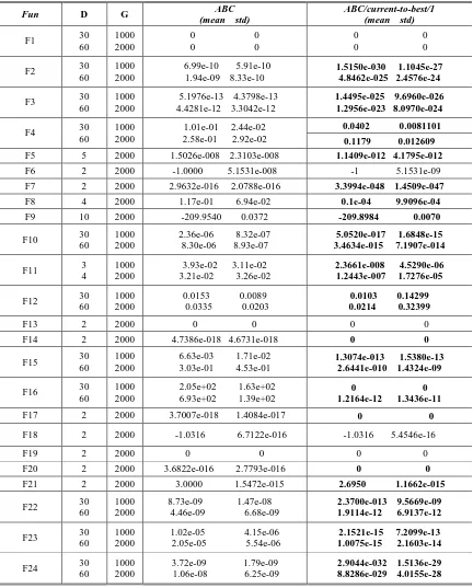
In the second experiment, parameters are arrange d below: population size SN is 100, limit is SN/2*D. All benchmark functions listed in Table 1 are condu cted for different dimensions. Each of the experime nt was run 30 times independently. The means and standard deviations of the experiments comparing o riginal ABC with that of we propose are reported in Table 3.

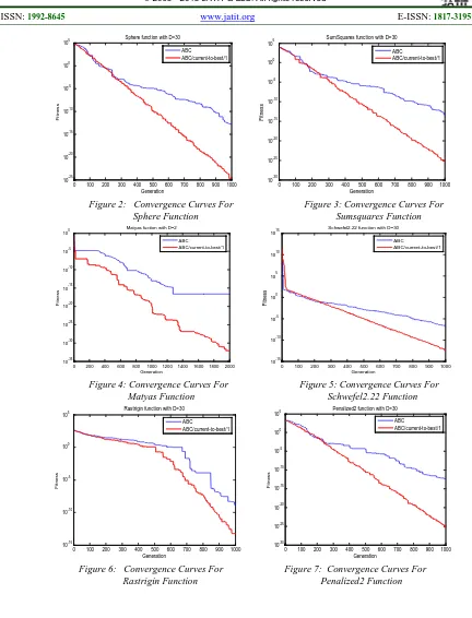
From the Table 3, we can see clearly that ABC/c urrent-to-best/1 displays preferable ability of search ing optimization in most cases through the searchin g space. In order to explain convergence speed mor e visually, we choose several benchmark functions t o illustrate it in Figure 2 - 7.

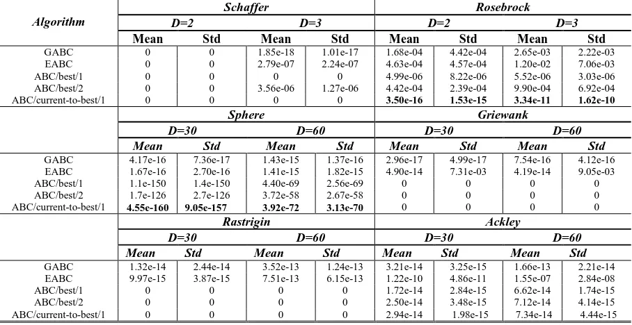
4.3 ABC/Current-To-Best/1 Vs. Other Pre-Existi ng Improved ABC

In this part, we will assess the performance of wh at we propose with GABC [13], ABC/best/1, ABC/ best/2[17], EABC [19]. The setting of parameters is the same as [13]. The result of the experiment is lis ted in Table 4 below.

[image:7.612.91.523.134.671.2]

Table 3. The Performance Comparison Of ABC And ABC/Current-To-Best/1

Fun D G ABC

(mean std)

ABC/current-to-best/1 (mean std)

F1 30

60

1000 2000

0 0

0 0

0 0

0 0

F2 30 60 1000 2000 6.99e-10 5.91e-10 1.94e-09 8.33e-10 1.5150e-030 1.1045e-27 4.8462e-025 2.4576e-24 F3 30 60 1000 2000 5.1976e-13 4.3798e-13 4.4281e-12 3.3042e-12 1.4495e-025 9.6960e-026 1.2956e-023 8.0970e-024 F4 30 60 1000 2000 1.01e-01 2.44e-02 2.58e-01 2.92e-02 0.0402 0.0081101 0.1179 0.012609 F5 5 2000 1.5026e-008 2.3103e-008 1.1409e-012 4.1795e-012 F6 2 2000 -1.0000 5.1531e-008 -1 5.1531e-09 F7 2 2000 2.9632e-016 2.0788e-016 3.3994e-048 1.4509e-047 F8 4 2000 1.17e-01 6.94e-02 0.1e-04 9.9096e-04 F9 10 2000 -209.9540 0.0372 -209.8984 0.0070 F10 30 60 1000 2000 2.36e-06 8.32e-07 8.30e-06 8.93e-07 5.0520e-017 1.6848e-15 3.4634e-015 7.1907e-014 F11 3 4 1000 2000 3.93e-02 3.11e-02 3.21e-02 3.26e-02 2.3661e-008 4.5290e-06 1.2443e-007 1.7276e-05 F12 30 60 1000 2000 0.0153 0.0089 0.0335 0.0203 0.0103 0.14299 0.0214 0.32399 F13 2 2000 0 0 0 0

F14 2 2000 4.7386e-018 4.6731e-018 0 0

F15 30 60 1000 2000 6.63e-03 1.71e-02 3.03e-01 4.53e-01 1.3074e-013 1.5380e-13 2.6441e-010 1.4324e-09 F16 30 60 1000 2000 2.05e+02 1.63e+02 6.93e+02 1.39e+02 0 0

1.2164e-12 1.3436e-11 F17 2 2000 3.7007e-018 1.4084e-017 0 0

F18 2 2000 -1.0316 6.7122e-016 -1.0316 5.4546e-16 F19 2 2000 0 0 0 0

F20 2 2000 3.6822e-016 2.7793e-016 0 0

F21 2 2000 3.0000 1.5472e-015 2.6950 1.1662e-015

F22 30

60

1000 2000

8.73e-09 1.47e-08 4.46e-09 6.68e-09

2.3700e-013 9.5669e-09 1.9114e-12 6.9137e-12

F23 30

60

1000 2000

1.02e-05 4.15e-06 2.05e-05 5.54e-06

2.1521e-15 7.2099e-13 1.0075e-15 2.1603e-14

F24 30

60

1000 2000

3.72e-09 1.79e-09 1.06e-08 6.25e-09

0 100 200 300 400 500 600 700 800 900 1000 10-25

10-20 10-15 10-10 10-5 100 105

Sphere function with D=30

Generation

F

it

nes

s

ABC ABC/current-to-best/1

0 100 200 300 400 500 600 700 800 900 1000 10-30

10-25 10-20 10-15 10-10 10-5 100 105

Generation

F

it

nes

s

SumSquares function with D=30 ABC

[image:8.612.90.522.66.632.2]

ABC/current-to-best/1

Figure 2: Convergence Curves For Figure 3: Convergence Curves For Sphere Function Sumsquares Function

0 200 400 600 800 1000 1200 1400 1600 1800 2000 10-35

10-30 10-25 10-20 10-15 10-10 10-5 100

Generation

F

it

nes

s

Matyas fuction with D=2 ABC ABC/current-to-best/1

0 100 200 300 400 500 600 700 800 900 1000 10-15

10-10 10-5 100 105 1010 1015

Generation

F

it

nes

s

Schwefel2.22 function with D=30 ABC

ABC/current-to-best/1

Figure 4: Convergence Curves For Figure 5: Convergence Curves For Matyas Function Schwefel2.22 Function

0 100 200 300 400 500 600 700 800 900 1000 10-15

10-10 10-5 100 105

Rastrigin function with D=30

Generation

F

it

nes

s

ABC

ABC/current-to-best/1

0 100 200 300 400 500 600 700 800 900 1000 10-30

10-25 10-20 10-15 10-10 10-5 100 105

Penalized2 function with D=30

Generation

F

it

nes

s

ABC ABC/current-to-best/1

[image:9.612.69.523.116.350.2]

Table 4. Performance Comparison Between ABC/Current-To-Best/1 And Pre-Existing Improved ABC

Algorithm

Schaffer Rosebrock

D=2 D=3 D=2 D=3

Mean Std Mean Std Mean Std Mean Std

GABC 0 0 1.85e-18 1.01e-17 1.68e-04 4.42e-04 2.65e-03 2.22e-03

EABC 0 0 2.79e-07 2.24e-07 4.63e-04 4.57e-04 1.20e-02 7.06e-03

ABC/best/1 0 0 0 0 4.99e-06 8.22e-06 5.52e-06 3.03e-06

ABC/best/2 0 0 3.56e-06 1.27e-06 4.42e-04 2.39e-04 9.90e-04 6.92e-04

ABC/current-to-best/1 0 0 0 0 3.50e-16 1.53e-15 3.34e-11 1.62e-10

Sphere Griewank

D=30 D=60 D=30 D=60

Mean Std Mean Std Mean Std Mean Std

GABC 4.17e-16 7.36e-17 1.43e-15 1.37e-16 2.96e-17 4.99e-17 7.54e-16 4.12e-16

EABC 1.67e-16 2.70e-16 1.41e-15 1.82e-15 4.90e-14 7.31e-03 4.19e-14 9.05e-03

ABC/best/1 1.1e-150 1.4e-150 4.40e-69 2.56e-69 0 0 0 0

ABC/best/2 1.7e-126 2.7e-126 3.72e-58 2.67e-58 0 0 0 0

ABC/current-to-best/1 4.55e-160 9.05e-157 3.92e-72 3.13e-70 0 0 0 0

Rastrigin Ackley

D=30 D=60 D=30 D=60

Mean Std Mean Std Mean Std Mean Std

GABC 1.32e-14 2.44e-14 3.52e-13 1.24e-13 3.21e-14 3.25e-15 1.66e-13 2.21e-14

EABC 9.97e-15 3.87e-15 7.51e-13 6.15e-13 1.22e-10 4.86e-11 1.55e-07 2.84e-08

ABC/best/1 0 0 0 0 1.72e-14 2.84e-15 6.62e-14 1.74e-15

ABC/best/2 0 0 0 0 2.50e-14 3.48e-15 7.12e-14 4.14e-15

ABC/current-to-best/1 0 0 0 0 2.94e-14 1.98e-15 7.34e-14 4.44e-15

5. CONCLUSION

In this paper, we modify the searching strategies of Artificial Bee Colony algorithm at the employe d and onlooker bees’ stage. The modification is ins pired by DE and introduces not only the best soluti on at the current generation but also stochastic pert urbation. We can get better balance between explo ration and exploitation by adjusting the amplitude of the perturbation f2 and f2.It is clear that the impr oved method we propose with suitable parameters can enhance the ability of searching optimization e ffectively by testing a group of 24 benchmark func tions.

ACKNOWLEDGEMENTS

The authors would like to express their gratitude to the anonymous reviewers for their valuable co mments and suggestions on this paper. This work i s supported by National Nature Science Foundatio n of China (Grant Nos. 61075049), the Excellent Young Talents Foundation Project of Anhui Provi nce (Grant Nos.2011SQRL018),the Youth Founda tion of Anhui University (Grant No. KJQN1015）, the University Natural Science Research Project o f Anhui Province(Grant Nos.KJ2012B038).

REFERENCES:

[1] Eiben, A. E. et al, “Genetic algorithms with mu lti-parent recombination", Proceedings of the I nternational Conference on Evolutionary Comp utation. The Third Conference on Parallel Prob lem Solving from Nature, October 9-14, 1994, pp.78–87.

[2] J.R. Koza, “Genetic programming: a paradigm for genetically breeding populations of comput er programs to solve problems”, Technical Rep ort STAN-CS-90-1314, Stanford University Co mputer Science Department, 1990.

[3] H.P. Schwefel, Kybernetische, “evolution als s trategie der experimentellen forschung in der st romungstechnik”, Master’s Thesis, Technical University of Berlin, Germany, 1965.

[4] Fogel, D.B. Fogel, L.J. Atmar, J.W, “Meta-evol utionary programming”, Proceedings of the tw enty-fifth Asilomar Conference on Signals, sys tems&computers, IEEE Conference Publishing

Services, November 4-6, 1991, pp. 540-545.

[5] Storn. R, Price. K, “Differential evolution–a si mple and efficient heuristic for global optimiza tion over continuous spaces”, Journal of global

optimization, Vol. 11, No. 4, 1997, pp. 341-35

9.

enetic and evolutionary computation, July 08 – 12, 2006, pp. 485-492.

[7] E. Bonabeau, M. Dorigo, G. Theraulaz, “Swar m Intelligence: From Natural to Artificial Syste ms”, Oxford University Press, NY, 1999. [8] Dorigo. M, Maniezzo. V, Colorni. A, “Ant syst

em: optimization by a colony of cooperating ag ents”, IEEE Transactions on Systems, Man, an d Cybernetics, Part B: Cybernetics, Vol. 26, N o. 1, 1996, pp. 29-41.

[9] R. Eberhart and J. Kennedy, “A new optimizer using particle swarm theory”, Proceedings of t he Sixth International Symposium on Micro Ma

chine and Human Science, October 4-6, 1995,p

p.39-43.

[10] X.S. Yang, “Engineering optimizations via nat ure-inspired virtual bee algorithms”, Artificial I ntelligence and Knowledge Engineering Applic

ations: A Bioinspired Approach, vol. 3562, No.

2, 2005, pp. 317–323.

[11] D. Karaboga, “An idea based on honeybee swa rm for numerical optimization”, Technical Rep ort TR06, Erciyes University, Engineering Fac

ulty, Computer Engineering Department, 2005.

[12] Srinivasan. D, Seow. T.H, “Particle swarm ins pired evolutionary algorithm (PS-EA) for multi objective optimization problems”, Proceedings of International Conference on Evolutionary C omputation, IEEE Conference Publishing Servi ces, Dec 8–12,2003,pp. 2292–2297.

[13] G.P. Zhu, S. Kwong, “Gbest-guided artificial b ee colony algorithm for numerical function opti mization”, Applied Mathematics and Computat ion, Vol. 217, No.7, 2010, pp. 3166–3173. [14] B. Akay, D. Karaboga, “A modified artificial b

ee colony algorithm for real-parameter optimiz ation”, Information Sciences, Vol. 192, 2010, p p. 120-142.

[15] B. Alatas, “Chaotic bee colony algorithms for global numerical optimization”, Expert Systems

with Applications, Vol. 37, 2010, pp. 5682–56

87.

[16] D. Karaboga, B. Basturk, “A comparative stud y of artificial bee colony algorithm”, Applied

Mathematics and Computation, Vol. 214, 200

9, pp.108–132.

[17] Weifeng Gao, Sanyang Liu, Lingling Huang, “A global best artificial bee colony algorithm f or global optimization”, Journal of Computatio

nal and Applied Mathematics, Vol. 236, 2012,

pp.2741-2753.

[18] S. Das and P. N. Suganthan, “Differential evol ution—A survey of the state-of-the-art,” IEEE

Trans. Evol. Comput, Vol.15, No.1, 2011, pp. 4

–31.

[19] E.M. Montes, et al, “Elitist artificial bee colony for constrained real-parameter optimization”, Proceedings of International Conference on Ev olutionary Computation, IEEE Conference Pub

lishing Services, July 18-23, 2010, pp.4244-69