QEH Working Paper Number 51
Emerging Stock Market Liberalisation, Total Returns, and Real Effects:
Some Sensitivity Analyses
J. Benson Durham*
Recent studies report that equity market liberalisation positively correlates with total return, which in turn purportedly increases private investment growth. While the finding on reform and performance is generally robust to alternative perspectives on capital account
liberalisation that emphasise over-heating and volatility, this crucial first link in the causal chain is not wholly robust empirically. For example, previous findings are very sensitive to alternative definitions of precise liberalisation event dates. Also, spatial variance seems to drive significant results in panel regressions, which is problematic for interpreting the particular path from equity prices to private investment. Finally, existing studies do not satisfactorily control for other determinants of returns, and extreme bound analysis (EBA) suggests that liberalisation is spurious.
October 2000
* Finance and Trade Policy Research Centre Queen Elizabeth House
University of Oxford Oxford OX1 3LA UK
1. Introduction
Whether capital account liberalisation has positive real macroeconomic effects in lower income countries is a considerably controversial issue. Nonetheless, despite the general dearth of evidence (Fischer, 1999), a few recent empirical studies report benevolent direct real effects of capital flows – including foreign direct investment (FDI)
(Balasubramanyam et al., 1996; Borensztein et al., 1998) and foreign portfolio investment (FPI) (Bekeart and Harvey, 1998) – on growth and private investment. Additional work focuses on indirect effects through financial variables such as stock market development and performance (Henry, 2000a, 2000b; Levine and Zervos, 1998b). This paper re-examines the short-run financial and, by implication, the real effects of stock market liberalisation through valuation.
Theory suggests that liberalisation, first, lowers the cost of equity capital and concomitantly produces an aggregate price appreciation, and, second, boosts private investment as erstwhile negative net present values (NPVs) become positive following reform. Several studies report a positive correlation between liberalisation and stock market performance (Henry, 2000a; Bekaert and Harvey, 1998; Froot et al., 1998), and fewer complete the transmission mechanism to private investment booms (Henry, 2000b). The policy implications for poorer countries are lucidly compelling – encourage stock market development, especially foreign equity inflows, and expect greater private investment (and growth).
But unfortunately, shortcomings beset the initial primary empirical link in the grand mechanism from reform to price appreciation to (private) investment. While the finding is generally robust given explicit controls for alternative and less optimistic perspectives on financial flows, particularly those that focus on over-heating and volatility, the statistical relation is highly sensitive to assessments of when the liberalisation event precisely occurs.
Also, problematic for the contention that corporate managers issue new equity at higher prices to fund investment after liberalisation, previous results on valuation heavily rely on spatial as opposed to temporal variance, as most individual time-series equations do not corroborate panel model results.
Leaving aside the appropriateness of event study methodology and interpretation of cross-sectional variance vis-à-vis adaptations of Tobin’s q related theory, the purportedly significant1 link between liberalisation and real total returns is not robust to alternative specifications. That is, liberalisation is not the only purported determinant of stock market performance. Rather, the literature on market anomalies is burgeoning, and previous
literature does not satisfactorily control for other factors. Therefore, following recent studies on stock market anomalies (Durham, 2000a, 2000b) and earlier literature on growth
regressions (Levine and Renelt, 1992; Sala-i-Martin, 1997a, 1997b) as well as the demand for money (Hess et al., 1998; Cooley and LeRoy, 1980), this paper uses extreme bound analysis (EBA) to determine specification bias. The results generally suggest that liberalisation is generally, as well as comparatively with respect to other factors, a spurious determinant.
Therefore, with respect to interpretation, the benevolent theoretical transmission mechanism from liberalisation to market performance to investment (and growth) is less persuasive if the first step is econometrically dubious. Of course, policy implications for poorer countries therefore are less straightforward. Perhaps stock market development does in fact positively affect long-run performance (Levine and Zervos, 1996, 1998a), a research question beyond the scope of this study, but the short-run implications of equity market reform for lower income countries remain unclear.
1
Unless otherwise noted, this paper uses ‘significant’ to mean statistical as opposed to economic significance, as outlined in McCloskey and Ziliak (1996). That is, a statistically significant parameter is distinct from the null hypothesis (of zero) according to some statistical test and (arbitrary) decision rule. Such a parameter is not necessarily economically significant, meaning the size of the parameter (the salience of the estimated impact) is meaningful for policy or theoretical implication.
Section 2 briefly outlines the general debate on the financial and real effects of international financial flows and capital account reform with particular respect to stock market liberalisation. Section 3 tests alternative perspectives on liberalisation. This includes explicit consideration of the alternative ‘boom-and-bust’ or ‘over-heating’ perspective, volatility in stock market returns, alternative liberalisation dates, and individual time-series regressions. Section 4 performs a broad sensitivity analysis of return in emerging markets and explores particular specifications under which liberalisation is fragile. Section 5 concludes.
2. Recent literature on equity market liberalisation and financial and real effects
FPI does not exhibit the advantages of FDI with respect to dissemination of
technology and (more arguably) capital flow stability according to conventional wisdom. But nevertheless, some economists advance the virtues of cross-border equity investment. For example, in his general overview of proposals for reducing global financial instability – including international bankruptcy courts, capital controls, and the prospect of a global central bank – Rogoff (1999) recommends a substantial shift from debt to equity finance. He argues that equity finance introduces risk sharing, via reductions in moral hazard with
ownership, as well as more efficient resource allocation, via (share) price signalling. His advocacy broadly reflects some recent studies (Levine and Zervos, 1996, 1998a) that produce a positive statistical correlation between aggregate stock market development measures (such as relative capitalisation, turnover, and volume) and long-run growth.
Similarly consistent with this benevolent perspective on stock market development and equity finance, recent literature suggests that stock market liberalisation – the decision to allow foreigners to investment in the domestic stock market – has positive real affects. For example, a (very) long-run perspective implies that reform encourages stock market
development, which in turn boosts macroeconomic performance (Levine and Zervos, 1996, 1998a, 1998b). While previous evidence perhaps curiously rests on samples that include OECD countries, 2 the tacit implication for lower income countries is that equity forms of FPI eventually produce sustained expansion.
Also, a second perspective, which is the focus of this paper, addresses the short-run effects of liberalisation on private investment through (windfall) increases in equity prices upon liberalisation. For example, Henry (2000a, 2000b) documents temporary increases in private investment growth rates among a sample of 11 developing countries3 that liberalised their stock markets during the 1977 to 1994 period (notably before the Tequila crisis). He argues that stock market liberalisation in general lowers the cost of capital, k,4 and therefore concomitantly increases aggregate stock prices in emerging markets.5 Given the decrease in
k and holding expected cash flows constant, some investment projects with negative NPVs
before liberalisation exhibit positive NPVs afterwards, which induces increased private
2
Durham (2000d) produces some evidence that suggests that data from developed countries largely drive the correlation between growth and stock market development.
3
These include Argentina, Brazil, Chile, Colombia, India, Korea, Malaysia, Mexico, the Philippines, Thailand, and Venezuela. He finds that in the first, second, and third years after liberalisation, 9, 10 and 8 of the 11 sample countries, respectively, had growth rates of private investment above their non-liberalisation medians. He reports that growth rates return to their pre-liberalisation by the fourth year after reform.
4
Henry cites three arguments that liberalisation lowers k (p. 2). First, ‘liberalisation can increase net inflows, which could reduce the risk free rate.’ Second, foreign participation in the domestic equity market ‘facilitates risk sharing across borders,’ which ‘should reduce the equity premium.’ Third, ‘increased capital inflows may also increase stock market liquidity,’ which purportedly reduces the equity premium. This contention is based on evidence that lower liquidity stocks have higher returns (Ahimud and Mendelson, 1986). He clearly notes, however, the possibility that the risk-free rate might rise upon liberalisation if ‘the autarky risk-free rate, which is an equilibrium outcome of aggregate savings and investment, is above or below the world rate’ (ft. 2). More generally, Henry suggests that ‘(t)he central message…is not that the stock market liberalisation will in all cases lead to a fall in a country’s cost of capital…(r)ather…stock market liberalisation may change the liberalising country’s cost of capital, with attendant implications for physical investment’ (p. 13, emphasis added).
5
One can easily deduce the effect of decreased k on aggregate prices from the standard Gordon growth model of aggregate valuation (in equilibrium), as in
P D
k g
=
− .
where D refers to dividends, k is the cost of capital (composed of the risk-free rate and the equity risk premium), and g is the expected growth rate of dividends. All else equal (most contentiously g in the case of
liberalisation), a decrease in k produces an increase in P. Of course, this formulation resembles the (mature) steady state and an equilibrium in which the growth rate is necessarily less than the cost of capital.
investment.6 Therefore, the short-run benevolent mechanism from flows through the stock market to the real economy follows:
(1)
L ib e ra liza tio n ⇒ ↓ ↑k, A g g r e g a teP ric e s⇒ ↑P riv a te In v e stm e n t .7 Notably, increases in private investment do not merely substitute for direct investment
according to previous evidence. Rather, Henry finds that the share of FDI to total investment in general increased (p. 19).8
Empirically, mechanism (1) of course implies two regularities. First, liberalisation must positively correlate with stock prices, and, second, such valuation changes should increase private investment. Notably, both dependent variables in this system – stock market behaviour and private investment – are hardly understudied. With respect to the first inquiry, without tracing the effects ultimately to private investment, many studies report a positive impact of flows on stock prices using distinct data sets as well as different observation frequencies.9 For example, Froot et al. (1998) report a positive correlation lagged equity capital flows and stock returns using daily data from 28 emerging markets from 1994 to 1998. Also, given lower frequency data and with varying degrees of qualification, Bekaert and Harvey (2000) and Henry (2000b) find that equity market liberalisation and/or flows
6
Another important issue, as Henry (2000a) readily suggests, is possible simultaneity bias, which the use of lower frequency data complicates. Given daily price and flow information, Froot et al. (1998) find evidence that, at least with respect to emerging markets, lagged flows help predict returns (pp. 3, 14). While they fail to control for broader global index performance, this broadly corroborates Henry’s contention that inflows lead to price appreciation (rather than vice versa).
7
It seems somewhat unclear from Henry’s (2000b) evidence whether liberalisation has a direct effect on private investment in addition to its (purported) gross effect on valuation. While he illustrates through statistical interaction terms that ‘liberalisation specific’ valuation changes have a significant effect on private investment, he never includes liberalisation and valuation simultaneously in any specification of private investment growth. If only gross liberalisation effects support the theory, then any lack of robust relation between reform and prices would be very problematic for (1).
8
The cost of equity capital, k, is related to local market volatility (variance) in closed capital markets. In open markets, k is related to the covariance with world market returns. Theory suggests that if the covariance is less than the (domestic) variance, then the cost of equity capital should decrease after liberalisation.
9 Portes and Rey (1999) find no relation between flows and returns using annual data and suggest that the dearth
lowers the cost of capital, as measured by ex post returns and/or dividend yields, in emerging markets.10
Regarding the second empirical question, the supposed link between price
appreciation and real variables is critical, as Henry documents a ‘strong correlation’ between the growth rate of investment and valuation changes, particularly stock price appreciation associated with liberalisation. As he notes, while some literature addresses this equation with respect to higher-income countries, there is a dearth of studies on lower income countries, and his (under-specified) regressions indicate that lagged one-year stock returns are significant determinants of private investment growth rates.11
The discussion now turns to evidence that supports the crucial first link in the causal chain.
3. Polemics on international capital flows:
Over-heating, volatility, liberalisation dates, and spatial variance
There are four shortcomings with respect to existing empirical estimations of equity market channels that broadly stem from the debate on capital account liberalisation. First, existing studies consistent with (1) do not satisfactorily test the ‘boom-and-bust’ hypotheses associated with more sceptical views of FPI, as there is a dearth tests that might capture the longer-run effects of liberalisation on possible over-heating and asset price bubbles. Second, studies do not control for volatility (absolute risk), which increases upon liberalisation
according to some studies (Levine and Zervos, 1998b). If volatility positively correlates with
10
In particular, Henry (2000b) finds that stock market liberalisation is a robust determinant of returns in equations that control for contemporaneous LDC, EAFE, and S&P500 index performance (p. 18). However, inclusion of macroeconomic fundamentals weakens the relation, as the dummy variables for trade and financial reform are no longer statistically distinguishable (p. 21).
11
Durham (2000d) also argues that controlling for other factors in the literature, namely lagged GDP growth, total private credit to GDP, government spending, and foreign exchange availability – vitiates the relation between lagged valuation changes and private investment growth. Moreover, he also finds that lagged valuation does affect private investment in developed markets.
(ex post) real total returns, as it should in (partially) segmented markets, such a relation would perhaps vitiate the purported (ex ante) decrease in k.
Third, unlike most event studies in econometrics, coding the event in question, stock market liberalisation, remains controversial. In fact, various studies use different dates, and, even more problematic, some economists argue that liberalisation is inherently a gradual process given uncertainty regarding policymakers’ commitment to sustainable reform (which might suggest that event studies per se are not necessarily appropriate). Put simply, a sturdy event relation between liberalisation and stock market returns (and therefore private
investment) should be robust to alternative dates based inherently on subjective assessments. Finally, cross-sectional variance considerably informs previous results, which is wholly sensible with respect to whether liberalisation affects returns. However, with respect to the particular transmission mechanism involving private investment decisions based on share prices, perhaps price appreciation vis-à-vis previous levels is more germane to corporate managers than relative stock market performance across space.
3.1. Sustainable asset price increases versus over-heating
Assuming a robust link between liberalisation and stock market performance, does liberalisation lead to sustainable increases in equity prices? Similar to Henry (2000a), Bekeart and Harvey (1998), and others, more pessimistic perspectives on capital account liberalisation also posit asset price increases (upon monetary expansion). However, such observers explicitly consider the prospect of overshooting, as financial bubbles eventually burst, and crises ensue (Calvo and Mendoza, 1999; Bhagwati, 1998).12 Therefore, to
12
Upon liberalisation, equity capital inflows could lead to rapid monetary expansion and a credit boom. Moreover, under a floating exchange rate, the demand for local currency should lead to considerable currency appreciation with potentially adverse effects on the trade balance. Under a fixed regime, the monetary authorities purchase of foreign currency could exacerbate monetary expansion (assuming no effective
sterilisation). In either case, some observers would expect resulting overheating, eventual reductions in output, and asset price contractions.
augment previous studies that document increases in aggregate prices, is there some
measurable cyclical symmetry to the initial appreciation? Put differently, how sustainable is the purported decrease in the cost of capital?13
Therefore, a useful econometric exercise is to test for lagged effects of liberalisation and flows on possible asset price collapses. Such a specification would not only address the one-time increase in prices (and decrease in k) but also consider the possibility of over-heating. The general model resembles
(2)
Rit = β0 +β1L IBtw +β2L IBtj +β3X +e
where Rit is the total aggregate real market return for country i at time t, LIB is the event
dummy for liberalisation, w refers to the event window before and including the
implementation month, j represents various intervals after liberalisation that might capture ‘over-heating,’ and X is a set of control variables. If β1 is positive and significant, consistent
with previous studies, but β2 is negative and significant, this would suggests that stock market
prices increase shortly after liberalisation but notably decrease after longer periods.
Depending of course on the relative values of β1 and β2, this result would seem to corroborate
the overheating perspective rather than the purely benevolent Tobin’s q14 related transmission mechanism from stock prices to private investment and the real economy. This inquiry addresses the longer-term effects of liberalisation as well as Bhagwati’s (1998, p. 10) general suggestion that advocates of capital mobility fail ‘to evaluate its crisis-prone downside’.
13
There is some econometric indication of this phenomenon. Bekaert and Harvey (2000) find some evidence, however sensitive to specification, that returns are lower in later periods following liberalisation. For example, they report that ‘(w)hereas we find a consistent decrease in dividend yields, excess returns may increase or decrease from the pre- to post-liberalisation period depending on specification. In the longer-term, average returns appear to be lower’ (p. 25). There are perhaps two conflicting interpretations. On the one hand, one could conclude that lower returns correspond with a lower equity premium and cost of capital. On the other, one might conjecture that in some cases, equity market liberalisation leads to price bubbles and market collapses.
14
Of course, changes in stock market prices only represent a portion of the numerator in Tobin’s q. Market value also includes debt securities.
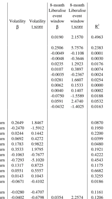
More specifically, evaluation of (2) in this paper includes the 8-month liberalisation window dummy to estimate β1, and X comprises proxies for global equity market
performance – including the MSCI USA index, the MSCI EAFE index, and an index for less developed countries (LDCs)15 – as well as country specific dummy variables. To inductively test for the possible effect of systematic overheating, j alternatively comprises various lag periods after liberalisation. As Table 1A indicates, these include 6-, 8-, and 12-month
intervals up to four years after liberalisation. For example, models 1 through 8 separately test for over-heating for every 6-month interval from the first month until the forty-eighth month after the event, and model 19 includes each of these post-liberalisation lags simultaneously, again, controlling for the liberalisation event window and X.
Turning to the results from Table 1A, 21 alternative forms of equation (2) fail to indicate any consistent overheating after liberalisation events,16 and importantly, the 8-month liberalisation window is clearly significant in all models, as the column of t statistics
indicates. While some intervals during the third and fourth years after liberalisation
(including models 6, 8, 12, 14, and 18) have negative coefficients, no parameter estimate is statistically significant.
Perhaps more surprisingly, some intervals covering various segments of the first year after liberalisation are (perversely) positive and statistically significant. For example, the interval from the seventh through the twelfth month after the event is significant (within the
15
The LDC index in this paper follows the IFC composite index, which dates from January 1985. The proxy for LDC index returns from January 1976 through December 1984 follows the market capitalisation weighted average of total returns for each available country in the IFC’s Emerging Markets Database. The correlation between this constructed proxy and the direct IFC composite index is 0.9957 using data from January 1985 through December 1997.
16
Similar to previous studies, panel regressions in this paper are temporally dominant, with considerably more time periods than cases. Therefore, similar to Durham (2000a, 2000b) econometric estimation follows FGLS with panel-corrected standard errors (Greene, 1997, pp. 651-654; Kennedy, 1998, p. 231; Beck and Katz, 1995), which entails OLS with its variance-covariance matrix estimated by (X'X)-1X'WX(X'X)-1, where W is an estimate of the error variance-covariance matrix. When T > N, the Parks-Kmenta method estimates the error variance-covariance matrix with insufficient degrees of freedom. The panel regressions also correct for possible panel-specific serial correlation using the Prais-Winsten transformation. The precise estimation command in STATA is ‘xtpcse’ with the option ‘c(psar1)’.
10 and 5 percent confidence intervals in models 2 and 19), and the larger estimate is nearly equal to the point estimate for the liberalisation window (0.0342 versus 0.0346, model 19). In addition, the dummy variable for the entire year after liberalisation is perhaps more clearly significant (models 15 and 21), although the point estimates are between 78 and 76 basis points lower than the liberalisation coefficient (models 15 and 21, respectively).
Economic interpretation of the apparent persistent positive effect after liberalisation seems somewhat problematic for the perspective on a one-time price appreciation outlined in mechanism (1). As this preliminary evidence indicates, perhaps the event window is even longer, extending not just before the announcement date due to information leaks, but also afterwards because market participants possibly assign a non-zero probability to a reversal of reform.17 In other words, evidence of delayed appreciation might reflect the perceived credibility of the stated commitment to liberalisation and the prolonged period required to convince the market that policymakers will successfully implement reforms.18
But in short, Table 1A most importantly indicates that increases in stock prices after liberalisation are largely sustainable, at least with respect to systematically consistent possible price collapses. These results certainly do not suggest, however, that market bubbles never develop after liberalisation. But, this empirical exercise uncovers no common trends in depreciation given this (limited) sample that is commensurable with previous studies.
3.2. Volatility, Liberalisation, and Returns
Another unexplored theoretical issue, also in the context of the debate on international capital flows, regards the simultaneously documented increase in stock prices (Henry, 2000b; Bekaert and Harvey, 2000; Froot et al., 1998) and augmentation in stock market volatility
17
This possibility might be analogous to the notion behind medium-term return momentum on the firm level, as market participants purportedly under-react to earnings announcements.
(Levine and Zervos, 1998b) after liberalisation. Again, several studies report a positive relation between reform and returns, but Levine and Zervos (1998b, p. 1182) also note that liberalisation tends to increase stock market volatility.19 Therefore, does the one-time increase in asset prices reflect the decrease in the cost of capital, or does the market simply compensate investors for the increased (absolute) risk? While variance is idiosyncratic in integrated capital markets, it is an appropriate risk measure in segmented markets according to theory (Bekaert et al., 1997, p. 45).20
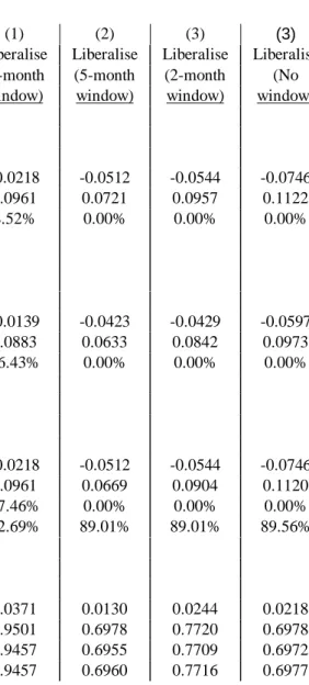
Indeed, as Table 1B illustrates, these data indicate a significant relation between volatility and liberalisation events.21 A panel regression of 12 emerging markets from January 1986 through December 1994, which replicates previous samples as closely as possible, suggests that volatility (the estimated standard deviation) increases on average by approximately 1.9 percent during the 8-month liberalisation window, which is significant within the 5-percent confidence interval (model 1).22 Also, a few individual (univariate) time-series regressions corroborate the relation, as data for Argentina suggest a 25.06 percent monthly increase in volatility upon liberalisation (model 2), and the equation for Thailand indicates a 5.91 percent increase (model 12). Finally, albeit at the 10 percent confidence interval, data indicate a 2.81 percent increase for Malaysia (model 8), but no other model yields significant results.
18
This perhaps reflects the potential bias in defining liberalisation events ex post. None of the events, for example, coded in Henry (2000a, 2000b) entail reform announcements followed by reneging of actual implementation.
19
The distinction between temporal and spatial variance with respect to this finding is noteworthy. While Levine and Zervos (1998b) find increases in volatility in individual time-series after liberalisation, they also note that with respect to the cross-section of stock markets that less integrated markets are more volatile (p. 1173). Furthermore, Bekaert (1995, p. 95) finds that market integration and volatility co-vary negatively, and Tesar and Werner (1995, p. 126) also report that the volume of equity flows from the United States also correlates negatively with volatility as well as market turnover. One might conjecture, then, that liberalisation might increase volatility in the short- run but decrease volatility in the long-run.
20
Markets might not be fully integrated after the liberalisation ‘event.’ Indeed, the very controversy
surrounding precise event dates (and therefore market segmentation) noted in Section 3.3 suggests that variance be an appropriate risk measure.
21
The calculations cover January 1986 through December 1994, which most closely matches Henry’s (2000b) sample, as data for all 12 countries are available during this period.
22
This significant correlation between volatility and liberalisation, which the panel regression documents and some time-series models corroborate, begs the question of whether previous models of return and liberalisation, such as (2), are under-specified and only capture the gross effect of the event, which might over-state its direct influences. More formally, the gross effect of liberalisation on stock returns, βG,R, follows
(3) βG,R = βD,R + (βD,V × αD,R)
where βD,R is the direct effect of liberalisation on returns controlling for volatility, βD,V is the
direct effect of liberalisation on volatility, and αD,R is the direct effect of volatility on return
controlling for liberalisation. Given that some evidence indicates that βD,V is positive,
estimates of αD,R would seem imperative, because a positive and significant coefficient would
suggest that βG,R overstates the effect of liberalisation on growth.23 This specification
question is perhaps of significant interest to observers that emphasise volatility in the context of international capital flows, and of course, simply controlling for absolute risk should shed light on this issue.
But notably, the data seem to indicate that the effect of volatility on return is ambiguous. Individual time-series models for Argentina and Korea suggest a positive and robust relation within the 10 and 5 percent confidence intervals, respectively (models 14 and 19), but the remaining parameters are insignificant. Moreover, data for Mexico, perhaps perversely, indicate a very strong negative effect (an approximate 0.7293 percent decrease in return per one percent increase in volatility) that is within the one percent confidence interval (model 21), and the corresponding panel regression for the 12 markets indicates no
significant effect (model 26). Finally, and perhaps most importantly, the direct estimate for
23 Put somewhat differently, consideration of the full system of equations helps indicate whether the indirect
αD,R indicates that volatility has no significant effect on return, controlling for liberalisation,
which is safely significant and positive within the 5 percent confidence interval (model 27). Therefore, these data suggest that the increase in volatility (variance) associated with liberalisation does not effect the apparent positive direct effect of reform on valuation. In fact, the indirect effect of liberalisation through volatility is insignificant, which broadly supports the perspective on k. One should note, however, that the key variable of interest in the context, volatility, is not measured directly but is an estimate following Schwert (1989, pp. 1117-1118) and Levine and Zervos (1998b). The preceding analysis would be more precise if daily total return data were available to estimate (non-overlapping) monthly volatility, but nonetheless, available data seem to support the first step in mechanism (1).
3.3. Alternative dates for ‘liberalisation’
While previous estimates of the effect of liberalisation on stock market performance often follow an event study methodology, researchers readily confess that, unlike other applications, the event in question is difficult to define (Henry, 2000a; Levine and Zervos, 1998).24 Estimates follow essentially historical analyses of reforms or more technical examination of structural breaks in the autocorrelation of cross-border equity flows, but the literature produces no consensus on when the crucial event in question occurs. The question, then, is whether findings with respect to stock market returns are robust to this
methodological controversy.
Some studies include some limited sensitivity analysis in this regard. For example, Henry (2000a) lists alternative liberalisation dates from various studies, and reruns the analysis coding for all ‘unique dates’ across four separate studies,25 and the exercise largely
24
Levine and Zervos (1998, p. 1173) write that ‘(s)electing…key dates when a country importantly changed policies toward international capital flows is both arduous and, ultimately, less systematic than we would like.’
25 That is, if two or more authors have two different liberalisation dates for the same cases, Henry assigns a
confirms his general findings. However, notably no study separately tests for each complete coding alternative. Toward that end, Table 1C lists the results for the baseline panel
regression using alternative event dates from Henry (2000a), Bekaert and Harvey (1998), Kim and Singal (1999), and Levine and Zervos (1998).
The data clearly suggests that the results are highly fragile to coding scheme. For example, with respect to the 8-month event window, both Henry’s coding and the unique dates from all four studies produce statistically significant results with the expected sign and general magnitude (rows 1 and 2). But, as rows 3 through 5 indicate, no other coding produces significant results within any conventional confidence interval. In fact, no scheme from Bekeart and Harvey (1998), Kim and Singal (1999), or Levine and Zervos (1998b) is significant for any event window given Henry’s (unbalanced panel) sample from January 1976 through December 1994. In fact, every coefficient using the dates from Levine and Zervos (1998b) is negative, which suggests a perverse effect. Therefore, in general these results imply that the significant empirical relation between liberalisation and returns depends critically upon (perhaps unsystematic) assessment of singular event dates.26
3.4. Temporal versus Spatial Variance
In general, supplementing panel regressions with time-series analysis helps indicate the relative importance of variance across time and space given a particular panel result. In fact, perhaps the issue of temporal versus spatial variance is particularly crucial with respect to the purported transmission mechanism from liberalisation to stock prices to private
investment levels. Of course, significant and positive cross-sectional findings with respect to liberalisation would indicate that, at any given point in time, a bourse that undergoes
liberalisation has greater total returns than non-liberalising markets. Conversely, time-series
26
evidence vis-à-vis the hypothesis would indicate that, irrespective of the particular case, total returns are greater in a given market during the 8-month liberalisation window compared to periods during which there is no such reform. As the panel regressions imply, both variance across space and over time is germane to the general question of whether liberalisation boosts stock market performance.
But, with more particular respect to the hypothesis regarding the effect on private investment, perhaps temporal variance is more germane. Again, the argument is that
managers in liberalising stock markets experience a decrease in k, NPVs increase, and private investment increases. Simply, it would seem that indigenous equity price changes with respect to previous local levels would be more relevant that the comparative performance of the local market vis-à-vis other foreign bourses.27 The relative temporal change in k seems to be critical according to theory, as NPVs turn from negative to positive notably over time, before and after reform.
Table 1D helps indicate the relative extent to which temporal and spatial variance inform the panel estimates. Notably, among 12 cases in the ‘baseline’ panel regressions, only the time-series regression for Colombia (which has only 120 observations), produces a
positive and significant coefficient for the 8-month event window within the 5 percent
confidence interval (model 9). The estimate for Malaysia is positive and significant at the 10 percent level (model 10), but the remaining 10 cases – Argentina, Brazil, Chile, India, Korea, Mexico, Thailand, the Philippines, Taiwan, and Venezuela – are clearly not robust. In fact, while again not significant, three cases – Chile, Mexico, and Venezuela – actually a negative effect of liberalisation. Therefore, perhaps problematic for the comprehensive mechanism from liberalisation to real variables, spatial variance seems to drive the overall panel result.
27 This should not be confused with the notion that k is related to the covariance (variance) of the local market in
4. Motivation for More General Sensitivity Analyses
Findings regarding the effect of stock market liberalisation and returns are robust to the boom-and-bust perspective and explicit consideration of the effect of reform on stock market volatility. However, the analysis nonetheless suggests that these findings are highly sensitive to the precise coding of when liberalisation occurs and whether cross-sectional variance informs the estimates. These findings cast some doubt on the short-run real effects of equity FPI in general and reform in particular.
But beyond the debate on capital account liberalisation, several studies suggest that many variables, seemingly unrelated to economic reforms, supposedly exhibit statistically significant relations with stock market performance. The literature on such anomalies is vast, which begs the question of whether previous findings regarding liberalisation, however sensitive to the issues raised in the previous section, are robust to broader specifications of the dependent variable. In addition, low overall fit measures for regressions in the previous section imply considerable unexplained variance, and therefore identification of possible missing variables seems prudent. But generally, how statistically significant is reform in the much broader context of the study of stock market behaviour?
4.1. Extreme Bound Analysis
As Durham (2000a, 2000b, 2000c) argues, the rigor of asset pricing studies is less advanced compared to sensitivity analyses of growth regressions,28 as very few studies satisfactorily control for competing explanations of market anomalies. With respect to the question of stock market liberalisation, the specification of real returns is sensible with respect to variables related to reforms, but nonetheless incomplete considering a much broader literature on market behaviour.
28 With respect to emerging market returns, Durham (2000a) finds that no emerging market factor is robust
Therefore, to help assess the relative robustness of the financial effects of
liberalisation, this section evaluates 14 additional anomalies germane to emerging markets studies using EBA. While the details of EBA with respect to this general research question can be found elsewhere (Durham, 2000a, 2000b) the basic framework follows
(4) Rit = αj + βzjz + βfjf + βxjxj + ε
where Rit is real total return, z is the ‘doubtful’ variable of interest, f is the set of ‘free’
variables that appear in every regression, and x includes variables from the set of 14 other ‘doubtful’ variables, χ. The EBA entails running M regressions that consider every possible linear combination of three variables from χ in x.29
Of course, the z variable of interest is liberalisation, using particular dates and event windows that produce significant results in (under-specified) previous studies. Following previous studies, f includes three aggregate equity indices – MSCI USA, MSCI EAFE, and the IFC (emerging market) composite – as well as country dummy variables (and a constant term).
With respect to χ, the sensitivity analysis should include most reasonable theories, and a very brief description of alternative hypotheses is instructive. For example, a sizeable literature examines value factors30 (Fama and French, 1998), and therefore the EBA employs
P/B, P/E, and D/P IFC ratios. Also, χ includes price history variables. The most simple and
succinct views include “contrarian” strategies in the short- (Jegadeesh, 1990)31 and long-term (De Bondt and Thaler, 1985), which exploit purported negative autocorrelations, and
“relative strength” strategies in the medium-run (three to 12 months), which utilise supposed
29
This follows Sala-i-Martin (1997a, 1997b) and, more importantly, a typical number of exogenous variables in multi-factor models of returns. Therefore, the total number of M regressions to evaluate the robustness of liberalisation vis-à-vis other variables is (14! ÷ [3! × 11!]) 364.
30
Members of the same family of factors are nonetheless independent variables. In fact, Fama and French (1998) note that, while value strategies, portfolios formed on P/B, P/E, D/P, and P/C are nonetheless distinct (p. 1985). An equation with sufficient degrees of freedom isolates the separate effects of variables from the same family.
positive autocorrelations (Asness et al., 1997). Turning to macroeconomics, as Bekaert et al., 1997 suggest, inflation should have a negative impact on cash flows, primarily via price signaling and operating cost shocks, and (univariate) empirical tests confirm the relation (Asprem, 1989). In addition, to capture published findings regarding population
demographics (Erb et al., 1997a), the EBA includes the lagged proportion of the population
older than 65. Furthermore, some researchers argue that survey measures of country risk correlate with stock returns,32 especially in emerging markets (Erb et al., 1995, 1996, and 1997b, Bekaert et al., 1997, Ferson and Harvey, 1997). Somewhat related, Bekaert et al. (1997) find that relative market size is significant, and Amihud and Mendelson (1986, 1991) argue that low-liquidity firms enjoy abnormal long-term returns within certain parameters. Also, non-equity financial development also conceivably relates to returns, as Demirgüç-Kunt and Levine (1996) find that stock market volatility significantly correlates with banking
system development. Finally, the doubtful set includes the January effect.
The first EBA purports to replicate previous samples as closely as possible. The data cover the same 11 emerging markets,33 but only from March 1987 because of data limitations on other variables in χ. To more closely replicate previous study and to therefore avoid capturing temporal out-of-sample bias, the data extend through December 1994. With 11 cases and 94 times periods, the total number of observations for the panel regressions is 1034.
4.2. EBA Results: Limited Sample
31
An important alternative perspective suggests that emerging markets in particular could exhibit positive autocorrelation, which would indicate predictability (Bekaert et al., 1997, p. 17).
32
Notably, these country risk measures might proxy for not only other concurrent reform policies but also for perceptions of credibility.
33
Given data limitations in the World Bank’s World Development Indicators, Taiwan is unfortunately not included in either EBA. Also, the earliest date for which data are available for all 11 countries and 14 χ variables is March 1987. This date notably follows liberalisation according to Henry’s coding for India (June 1986) and the Philippines (May 1986), two cases that nonetheless inform the EBA estimates. While some authors (Bekaert and Harvey, 1998; Kim and Singal, 1999) do code liberalisation dates for both countries during the EBA sample period, the inclusion of markets that did not liberalise would seem to usefully inform estimates
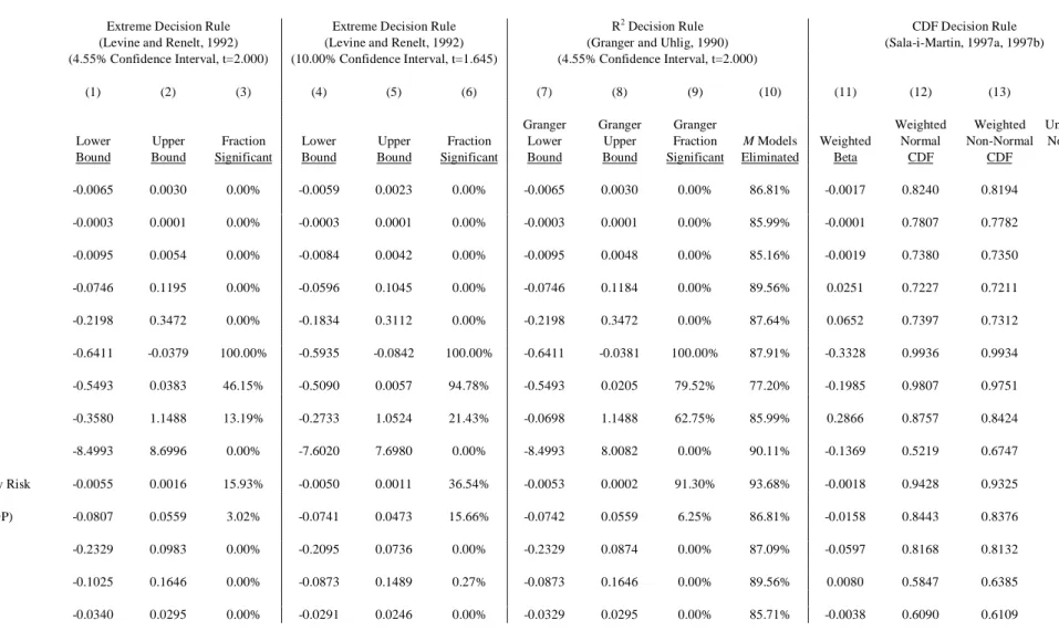
In general, EBA suggests that liberalisation is not in fact a robust determinant of stock market performance.34 For example, as Table 2A indicates, the 8-month window for
liberalisation does not pass the ‘extreme’ decision rule.35 With respect to both the 4.55 and 10 percent confidence intervals, the upper and lower bounds have the opposite signs (column 1, rows 1-2, 4-5, respectively), and the coefficient is only significant in approximately 8.52 and 46.63 percent of all (364) M regressions.36 Also, given elimination of models not within 90 percent of the specification that explains the most variance (following the R2 decision rule), only 17.46 percent (row 9) of the coefficients are significant, and the bounds have opposite signs (rows 7-8). Finally, while the weighted beta is positive and comparable to of whether the event affects the dependent variable. (Perhaps all stock markets should be included in any analysis of the effect of cross-sectional variance in liberalisation events.)
34
The regression that omits every variable from χ but controls for world market proxies and country specific effects suggests that the 8-month liberalisation measure is significant at the 10 percent level. Specific details on all underlying models are available on request.
35
For a more complete description of EBA decision rules see Durham (2000b), but the three basic rules used in this paper are as follows. The ‘extreme’ decision rule (Levine and Renelt, 1992) essentially states that each t statistic among the M regressions should be greater than 2 (or 1.645 using the 10 percent confidence interval as Henry does), and each z coefficient should have the same sign. A more lenient criterion (Granger and Uhlig, 1990) suggests that only models among the original M regressions with an R2j that satisfies
R2j≥ (1-α)R2max
where R2max is the highest R2 value among all M regressions, and α is 0.1 in this study. This ‘R2’ decision rule is
identical to the extreme criterion, but only models that satisfy the condition inform the bounds. Finally, the ‘CDF’ decision rule follows the test outlined in Sala-i-Martin (1997a, 1997b). Sala-i-Martin weights each of the M estimates of βz by some measure of overall fit for the underlying jth regression. The weighted means in this paper follow βz zjβzj j M = =
∑
w 1 and σ2 σ2 1 z zj zj j M = =∑
w where wzj is the weight, as in∑
= = M i zi zj zj R R w 1 2 2 .36 The 8-month event window is perhaps the most apt to pass a EBA decision rule among the liberalisation
measures. As Henry (2000a) suggests, the event window perhaps more realistically captures the flow of information regarding imminent reform. But a remaining problem is that policymakers are considerably more inclined to liberalise when market performance is relatively (presumably with respect to temporal variation) positive, thereby making the empirical link between the event window and returns possibly endogenously selected. (Policymakers would not wish to open equity markets and sell shares at ‘fire sale prices’ to foreigners following periods of poor market performance.) Seemingly, the longer the event window, the more problematic
previous estimates at approximately 3.71 percent (Henry, 2000a), the figure only passes the CDF decision rule under the assumption of weighted normality (row 12). The weighted non-normal (row 13) and un-weighted non-non-normal (row 14) assumptions narrowly miss the decision rule.37
The remaining measures of liberalisation using alternative event windows produce more unequivocally fragile results. In fact, as all statistics under the extreme and R2 decision rules indicate, no liberalisation coefficient is robust controlling for any x set of three χ factors, even with the 10 percent confidence interval (row 6, columns 2-4). Of course, all statistics germane to the CDF decision rule similarly indicate fragility, as the weighted betas, while positive in support of the hypothesis, are considerably lower than the 8-month window estimate (3.71 percent) (row 11, columns 2-4).38
4.3. EBA Results: Expanded Sample
Unfortunately, previous studies seem with respect to temporal coverage through 1994, which perhaps notably precludes key crises in emerging markets, including the Tequila Crisis in Mexico the Asian Flu beginning in 1997. This section present results from an expanded sample that includes 5 additional countries from regions beyond Latin American and East Asia – Greece, Jordan, Nigeria, Pakistan, and Zimbabwe – and data on all countries through the end of 1997. Liberalisation dates for the additional five countries follow Bekaert and Harvey (1998). Notably, this panel produces a considerably more powerful test, as the
possible endogenous selection, but the more likely a significant result (in an EBA). (Indeed, a review of Henry’s results for alternative windows suggests that the relations are more robust for longer windows.)
37
This study notably does not consider other reforms – with respect to trade, stabilisation, exchange rate controls, and privatisation – that might occur simultaneously with equity market reform. This would suggest that the following EBA is somewhat biased toward positive and robust results for liberalisation. (Henry’s precise monthly coding for these other reforms was not made available.)
38
EBA also indicates that post liberalisation effects reported in Table 1A are also sensitive to specification. Only one regression among the 364 possible models (which include the 8-month liberalisation window in f along with the MSCI USA, MSCI EAFE, and IFC indices) is significant at the 10 percent level for the measure that considers the seventh through the twelfth month after liberalisation. Only 2.2 percent of models for the variable covering the first year after the event are statistically significant. Results are available on request.
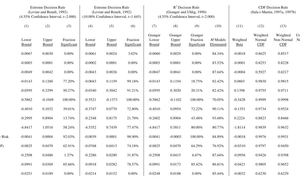
number of observations more than doubles from 1034 to (16 countries × 130 months) 2080. As a result, the EBA also illustrates ‘out-of-sample’ in addition to specification bias vis-à-vis previous literature. But nonetheless, an applicable finding should be robust across space, time, and specification assumptions.
Turning to the results, Table 2B again suggests that liberalisation is not a robust correlate of stock market returns.39 For example, the standard 8-month window clearly passes no decision rule, as the coefficient is significant in only 1.65 percent of the 364 regressions at the 4.55 percent confidence interval and only 22.25 percent at the 10 percent level. The R2 and CDF decision rules similarly indicate fragility.
The alternative 5-month liberalisation window seems more robust, as 4.12 and 46.98 percent of the M coefficients are significant at the 4.55 and 10 percent confidence intervals. But, the upper and lower bounds have opposite signs, only 1.61 percent of superior models are significant (row 9, column 2), and CDF statistics narrowly miss the decision rule. Finally, the 2-month event window and contemporaneous implementation measures are insignificant in all possible specifications and therefore fail all EBA decision rules.
4.4. Complete EBA of Anomalies in Emerging Markets
All in all, liberalisation measures are not robust to EBA. None of the event windows around reform dates are robust according to any decision rule in either the limited or
expanded panel samples. But, as previous applications of EBA to financial market anomalies (Durham, 2000a, 2000b, 2000c) and other econometric issues (Levine and Renelt, 1992; Sala-i-Martin, 1997a, 1997b; Hess et al. 1998) indicates, very few independent variables tend to pass the extreme decision rule. While stock market liberalisation indeed fails more lenient
39
With respect to the augmented sample, the regression that omits every variable from χ but controls for world market proxies and country specific effects suggests that the 8-month liberalisation measure is in only
significant at the 12 percent level. This suggests that in addition to specification, fragile results are also due to out-of-sample bias.
EBA tests, the question remains as to whether any other variables in the remaining set of doubtful variables, χ, are robust. In other words, how comparatively robust is liberalisation compared to other purported determinants of stock market returns? Is EBA too stringent a test? Also, in addition to statistical significance and specification, are other variables also economically significant?40
Tables 3A and 3B address this issue and summarise the EBA results for all 14 variables in the χ set for the limited and expanded samples.41
Similar to the results for liberalisation summarised in Table 2B, these data suggest that some variables are also fragile according to all EBA decision rules under identical test conditions. These variables include
value measures (P/B, P/E, and D/P), inflation volatility, market capitalisation, market liquidity, and the January effect.
However, in sharp contrast to liberalisation, a number of variables pass at least one EBA criterion in at least one sample and additionally exhibit economic significance. For example, the long-term contrarian proxy is significant in every M specification and therefore passes the extreme decision rule (and therefore the remaining tests) in both the limited and more comprehensive sample. Moreover, the weighted beta from the augmented (limited) sample of approximately 0.3438 (0.3328) percent listed in Table 3B (Table 3B) has the expected sign. Inflation has the expected negative aggregate coefficient and passes the CDF
40
Following McCloskey and Ziliak (1996), this section duly notes the size of the weighted betas to address the distinction between statistical and economic significance, which some applications of EBA neglect given its explicit emphasis on the former.
41
There are a few key differences between the EBA of emerging markets in Durham (2000a) and the present study. First, the augmented sample differs considerably with 2080 versus 1328 panel observations, as this study includes data from March 1987 through December 1997, while the previous study covers March 1988 through January 1995. The number of cases is similarly 16, but this study substitutes data for Portugal with data covering Jordan. Second, the previous study includes temporal dummy variables to capture shocks, whereas this study includes market proxies for the U.S., EAFE, and a LDC (IFC) index, which follows Henry (2000a). Third, given that the emphasis in this sensitivity analysis is not to capture replicable investment strategies, some variables enter the current study contemporaneously, including inflation, inflation volatility, country risk, population demographics, and bank development. Fourth, the measure for inflation volatility follows Schwert (1989) rather than the relative change in inflation rates from month to month. Fifth, the previous study uses total nominal excess ($U.S.) return on the left-hand-side, while the dependent variable in this study is the total real gross ($U.S.) return. While the overall EBA results are similar, these key differences may contribute to the generally more robust results in this application of EBA.
criterion in both samples, as the weighted beta suggests that a one percent increase in the monthly inflation rate corresponds with a 0.1351 (0.1985) percent decrease in real monthly ($U.S.) total return in the augmented (limited) sample.
Also, at least with respect to the augmented sample, five other ‘doubtful variables’ are robust, at least in the augmented sample. The Institutional Investor country credit rating narrowly misses the extreme decision rule, but passes the R2 and CDF criteria with the expected coefficient. The weighted coefficient suggests that the difference between the lowest (Nigeria in March 1996 and March 1997) and highest country credit rating (Korea in October 1995) implies an approximate 10.332 percent monthly increase in total returns. Four other factors pass the CDF decision rule in the augmented sample. The weighted beta for
momentum suggests that monthly total returns are approximately 0.1398 percent greater.
Also, a one percent increase in the proportion of the population older than 65 suggests a 1.8114 percent decrease in return, and a one percent increases in the ratio of bank credit to GDP suggests an approximate 4.21 basis point decrease in return. Finally, the short-term
contrarian proxy is robust to Sala-i-Martin’s test statistic. The weighted coefficient suggests
that a one percent increase in the previous month’s total return corresponds with an approximate 6.02 basis point contemporaneous increase, which is inconsistent with the contrarian hypothesis but corroborates the view of emerging market inefficiency (predictability).
In general, these results on other (competing) perspectives on stock market performance suggests that EBA is not an unreasonable econometric criterion on which to doubt results on stock market liberalisation. Clearly, especially given the augmented sample, other factors are robust in identical samples, as seven variables pass EBA tests in at least one sample. Also, while assessments as to ‘how large is large’ are ultimately subjective
particularly including long-run lagged returns, inflation, country risk, and population demographics – seem noteworthy. Therefore, one might conjecture that specification bias besets results for liberalisation.
4.5. Toward identification of problematic specifications
Previous applications of EBA (Levine and Renelt, 1992; Sala-i-Martin, 1997a, 1997b; Hess et al. 1998; Durham, 2000a) do not discuss particular specifications that produce fragile results for particular hypotheses of interest. They simply report the robustness of each doubtful variable. But, perhaps some preliminary discussion of key specifications that are problematic might be instructive for future research. The fragility of stock market
liberalisation is of course no exception, and therefore this section examines which, if any, variables in χ drive insignificant coefficients for liberalisation measures.
Toward that end, Table 4A lists summary statistics for sub sets of the M regressions from Table 2A by doubtful variable. For example, row 6 lists 9 statistics for all 78 equations (among the total 364 models) that include the long-run contrarian proxy. Row 6, column 2 indicates that of the 78 regressions which include long-run lagged returns, 23.08 percent produce statistically significant coefficients for the 8-month liberalisation measure at the 10 percent confidence interval. Given that liberalisation is significant in 46.43 percent of specifications overall (Table 2A, row 6, column 1), inclusion of this particular doubtful variable further increases the probability of an insignificant coefficient for liberalisation. Similarly, column 1 suggests that including inflation volatility (row 8), country risk (row 10), and relative market size (row 11) are particularly problematic, as only 7.69, 7.69, and 35.9 percent of the regressions produce significant results for liberalisation, respectively.42
42
The average t statistic captures similar information, as the figures for variables that produce no significant coefficients, inflation volatility and country risk, are the lowest among the 14 factors at approximately 1.46 and 1.44, respectively.
Also, Table 4A indicates which particular specifications produce the extreme bounds. For example, the model that includes the long-run contrarian proxy, inflation volatility, and country risk in the x set produces the lower bound (column 3), and the equation that includes inflation, turnover, and bank development produces the upper bound (column 4). Perhaps also instructive, Table 4A also shows which model among the 364 regressions has the best overall fit, as the model that includes the long-run contrarian proxy, inflation, and inflation volatility has an R2 value of 0.1302. Notably, liberalisation is not significant in this particular regression within any standard confidence interval, with a t statistic of only 1.388.43
The expanded panel sample produces similar results. For example, variables that are particularly problematic for the 8-month window measures include the long-run contrarian proxy (12.82 percent significant at the 10 percent confidence interval – Table 4B, row 6, column 2), inflation volatility (1.28 percent), population demographics (0.00 percent),
country risk (0.00 percent), and relative market size (10.26 percent). Also, the model among the 364 M regressions with the best fit includes long-run lagged returns, inflation, and
country risk, and notably, the 8-month widow has the expected positive sign, but the parameter is insignificant with a t statistic of 1.251.44 Finally, as Table 4C indicates, the same five variables similarly seem to increase the probability of fragile results for the 5-month window, and the best model again produces an insignificant result for liberalisation (t statistic of 1.34).45
Therefore, while liberalisation is largely fragile according to EBA inference criteria, this examination of subsets of M regressions by (competing) doubtful variable indicate that some factors seem to increase the probability of insignificant results. Perhaps future research
43
Long-run lagged returns and inflation significantly enter the equation with the expected negative signs and t statistics of 2.656 and 2.547, respectively. Inflation volatility is unexpectedly positive, with a t statistic of 1.935. Further particulars on all M regressions are available on request.
44
In this particular model, each variable included in x is statistically significant with the expected sign, and the R2 value is 0.094 (Table 4B; rows 6, 7, 10; column 9).
should consider particular variables such as inflation, long-run lagged returns, country risk measures, and relative market size.
4.6. Time-Series EBA
Several factors recommend supplementing panel regressions with time-series analysis of individual countries. In addition to isolating the general importance of spatial and
temporal variance, time-series analysis ameliorate problems in defining concepts across different markets, as variables such as accounting measures or, particularly given this research question, liberalisation. Again, as Table 1C indicates, definitions of the event in question are highly contentious, and the results are very sensitive to definitional changes.
Given the fragility outlined in the previous section, time-series EBA is also
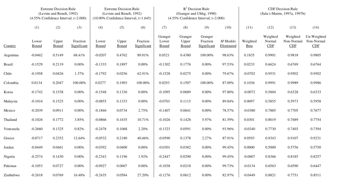
instructive, and Table 5A summarises the results for 14 countries from the expanded panel sample that covers March 1987 through December 1997. Notably, few time-series results support the liberalisation hypothesis, as data from only two countries are robust according to any decision rule with the expected sign. Data for Colombia do unequivocally suggest that liberalisation leads to higher real returns, as the variable is clearly robust according to the most extreme decision rule with a weighted beta that implies approximately 10.36 percent greater returns on average during the 8-month event window. Also, some data for Argentina support the hypothesis, as the coefficient suggests 18.35 percent greater returns given
liberalisation, which passes the R2 and CDF but not the extreme decision rule.46
But the remaining 12 cases clearly do not support the hypothesis. In fact, data for Brazil, Korea, Malaysia, Mexico, Thailand, and Venezuela, all suggests that temporal
variation in liberalisation is fragile. Also, countries notably excluded from previous samples
45
Similar to the results for the 8-month window in the expanded panel sample, the equation that includes the long-run contrarian proxy, inflation, and country risk produces the greatest overall fit, as each factor is safely significant with the expected sign.
(Henry, 2000b) – Greece, Jordan, Nigeria, Pakistan, and Zimbabwe – all indicate that
liberalisation does not pass any EBA decision rule. Perhaps most problematic, however, data for Chile actually indicate a negative effect on returns during the 8-month window, which is robust at least according to the CDF decision rule.
5. Conclusions
The recently reported positive association between equity market liberalisation, stock prices (the decrease in k), and private investment has profound implications for lower income countries. Assuming robust empirical relations to support this transmission mechanism, (nascent) emerging stock markets should allow foreigners to purchases domestic shares, and policymakers can expect price appreciation and increased private investment. In some respects, this paper suggests that previous evidence is robust to controversies in the literature on international capital flows. That is, at least with respect to the first chain in the
mechanism, liberalisation seems to lead to sustainable increases in equity price levels given models that include post-liberalisation dummy variables – booms do not seem to be followed by busts. Also, the effect of liberalisation on prices seems independent from its effect on market volatility, which does not seem to affect performance.
But unfortunately, other sensitivity analyses cast doubt on the benevolent relation. For example, the event study methodology on which these findings are based ultimately rests on subjective assessments of when ‘liberalisation’ exactly occurs. Indeed, this paper shows that previous results are extremely sensitive to alternative sets of event assumptions. Also, even using coding that produces significant results, it seems that spatial as opposed to
temporal variance seems to drive previous findings from panel regressions, as only data from only one country, Colombia, suggests a statistically significant result within the 5 percent
46 Table 5B1 indicates that liberalisation would pass the extreme decision rule using data for Argentina if only
confidence interval. Briefly, while spatial variance is in fact relevant to the general question of whether liberalisation effects prices, it seems less relevant to this particular transition mechanism from local market price appreciation to private investment growth.
Moreover, event definitions and spatial variance aside, liberalisation is not the only purported determinant of stock market performance according to the empirical finance literature. In fact, EBA analysis indicates that the hypothesis is not robust to alternative specifications. Notably, while EBA is a rigorous exercise, this paper nonetheless shows that some variables are in fact robust to various decision rules, which suggests that liberalisation is comparatively fragile. Perhaps useful for future empirical research and theory, inclusion of a few particular variables – the long-run contrarian proxy, inflation volatility, population demographics, country risk measures, and relative market capitalisation – seem to increase the probability that liberalisation is statistically fragile.
Therefore, the statistical relation between liberalisation and stock market performance is perhaps not as lucid as previous studies suggest. This implies that the grand transmission mechanism from reform to private investment growth is empirically tenuous, especially if liberalisation has no direct effect on private investment in addition to its purported gross effect through valuation. While the evidence in this paper does uncover robust negative effects, the short-run policy implications of stock market liberalisation seem unclear.
Two questions remain with respect to interpretation, particularly with respect to policy. First, given persuasive theory, ambiguous results require some explanation.
Therefore, to briefly proffer a possible interpretation, as other economists discuss in detail, policymaker credibility could be critical in this regard. Under textbook conditions
policymakers are fully committed to reform and market participants have perfect information through the announcement, and this reform scenario should produce a one-time decrease in k and increase in stock market prices. But, if the market does not consider reform
pronouncements as credible, prices are unlikely to respond accordingly, all things being equal, and indeed, the use of event windows in previous studies seems to accommodate market imperfections by definition. Therefore, ambiguous results given more fully specified models of asset returns might reflect market participants’ perception of reform credibility and commitment.47 Simply, equity markets may not judge policy as credible, and reform
announcements therefore have no robust measurable effect on prices.48
Second, general conclusions from the evidence in this paper regarding the real effects of stock markets in lower income countries can only be drawn with considerable trepidation, as this study only address the first phase in the short-run mechanism. However, some data suggest that liberalisation does not directly affect private investment, controlling for several factors in the literature as well as contemporaneous and lagged valuation changes (Durham, 2000d). Also, some long-run data suggest that the correlation between stock market
development and economic growth only holds for higher income country samples (Durham, 2000d), which casts doubt on the second phase of the long-run mechanism from reform to expansion. But these issues aside, which are far beyond the scope of this paper, the relation between liberalisation and market returns seems questionable, and therefore lower income countries should proceed cautiously with reform.
47
Perhaps the comparatively robust findings for inflation according to the CDF EBA decision rule in both the limited and expanded samples is germane to policy credibility – markets seem to react favourably to lower inflation.
48 Some intervening factors might be relevant. For example, it might be instructive to explicitly consider the