Feature Selection by Joint Graph Sparse Coding
Xiaofeng Zhu
∗and Xindong Wu
†and Wei Ding
‡and Shichao Zhang
§Abstract
This paper takes manifold learning and regression simulta-neously into account to perform unsupervised spectral fea-ture selection. We first extract the bases of the data, and then represent the data sparsely using the extracted bases by proposing a novel joint graph sparse coding model, JGSC for short. We design a new algorithm TOSC to compute the resulting objective function of JGSC, and then theoretically prove that the proposed objective function converges to its global optimum via the proposed TOSC algorithm. We re-peat the extraction and the TOSC calculation until the value of the objective function of JGSC satisfies pre-defined condi-tions. Eventually the derived new representation of the data may only have a few non-zero rows, and we delete the zero rows (a.k.a. zero-valued features) to conduct feature selec-tion on the new representaselec-tion of the data. Our empirical studies demonstrate that the proposed method outperforms several state-of-the-art algorithms on real datasets in term
of thekNN classification performance.
1 Introduction
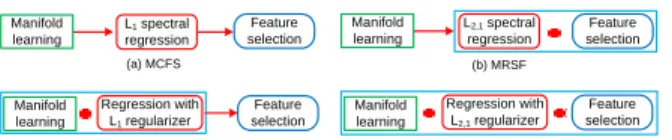
Feature selection is an effective solution to the high-dimensionality problem in real applications. Recent studies on spectral feature selection have integrated manifold learning into features selection. Spectral feature selection can improve the performance of feature selection because it preserves the local structures of the data via manifold learning. However, most existing efforts are designed to sequentially conduct manifold learning and regression. For example, the MCFS method in [2] (see Fig. 1.(a)) includes two key steps, manifold learning and spectral regression respectively. After performing manifold learning, i.e., performing locality preserving projection (LPP), MCFS conducts spectral regression one eigenvector at a time to generate the element sparsity (see Fig. 2.(a)). Then a new score rule is designed to rank the goodness of the features (with the element sparsity). At last MCFS performs feature selection by deleting the features with low score values.
∗The University of Queensland, Australia †The University of Vermont, USA
‡The University of Massachusetts Boston, USA §Guangxi Normal University, China
Manifold learning L1 spectral regression Manifold learning L2,1 spectral regression Regression with L1 regularizer Manifold learning Regression with L2,1 regularizer Manifold learning Feature selection Feature selection Feature selection Feature selection (a) MCFS (c) GSC (d) JGSC (b) MRSF
Figure 1: Methods on spectral feature selection. MCFS has the following limitations. Firstly, the element sparsity is ill-fitted for feature selection. Given an example shown in Fig. 2.(a), according to the score rule in MCFS, the second row will be the first feature to be deleted for feature selection. However, the non-zero values in the second row (i.e., 0.51, 0.23, 0.45 and 0.58) will be lost. It is obvious that no matter which row is deleted, the non-zero values in that row will be lost since the element sparsity does not generate zero elements through the whole row, which is different from the row sparsity illustrated in Fig. 2.(b). Secondly, MCFS conducts spectral regression one eigenvector at a time, thus it does not consider the correlations among the spectral features. Recent studies (e.g., [15]) have shown that evaluating the spectral features individually cannot effectively identify redundant features. Thirdly, the performance of MCFS can be further improved by simultaneously performing manifold learning and regression, such as the GSC and JGSC methods (see Fig. 1.(c) and Fig. 1.(d)). Existing literatures (e.g., [3, 16]) have shown that simultaneously considering manifold learning and regression results improved performance in learning, e.g., classification or clustering.
Zhao et al., [15] proposed the MRSF algorithm (see Fig. 1.(b)) to perform spectral regression after conducting manifold learning. MRSF uses the ℓ2,1
-norm regularizer to replace the ℓ1-norm regularizer in
MCFS. As illustrated in Fig. 2, the row sparsity used in MRSF obviously fits better for feature selection than the element sparsity used in MCFS. However, MRSF only solves the first two problems of MCFS but does not address the third one.
Recently graph sparse coding (GSC) [3, 16] (see Fig. 1.(c)) embeds manifold learning into the reconstruction process. It has been shown that GSC achieves improved performance in real applications. Due to employing
0 0 0 0 0 0.91 0.85 0.23 0.15 0.58 0 0 0 0 0 0.56 0.24 0.85 0.24 0.84 Codes 0 0.65 0.67 0 0.48 0.51 0 0.23 0.45 0.58 0 0.75 0 0.82 0 0.56 0 0.69 0.34 0 Codes
(a) The element sparsity (b) The row sparsity Figure 2: An illustration to compare the element sparsity (via the ℓ1-norm regularizer) with the row
sparsity (via theℓ2,1-norm regularizer).
theℓ1-norm regularizer for achieving the sparsity, GSC
generates the element sparsity (see Fig. 2.(a)). GSC only focuses on the third problem of MCFS and does not address the first two issues. Moreover, GSC is designed for clustering [16] and classification [3] rather than feature selection.
In this paper we discuss a new feature selection method to overcome the drawbacks of MCFS. Motivated by existing studies (e.g., [2, 3, 15, 16]), we model feature selection as a novel joint graph sparse coding model (JGSC). The proposed JGSC (see Fig. 1.(d)) is designed to simultaneously perform manifold learning and regression as well as to achieve the row sparsity. In particular, JGSC consists of three key steps: 1) Basis extraction. The bases are derived from the data via an existing dictionary learning method, such as [8]. 2)
Data reconstruction. The data is reconstructed into the derived basis space to generate its new representation using the proposed new joint graph sparse coding model. We repeat these two steps (i.e., basis extraction and data reconstruction respectively) until the value of the objective function of JGSC satisfies pre-defined conditions. 3) Feature selection. Due to introducing the ℓ2,1-norm regularizer, the derived representation of
the data contains many zero rows. This shows that the zero rows (a.k.a. zero-valued features) of the new representation of the data are unimportant. To achieve efficiency and effectiveness, we delete those rows to obtain a reduced dataset.
We summarize the contributions of this paper as follows:
• We identify limitations existing in traditional spec-tral feature selection, mainly caused by unavoidable drawbacks of MCFS discussed above. We devise an effective solution to tackle the limitations via the proposed joint graph sparse coding model by si-multaneously performing manifold learning and
re-gression (between the original data and the bases, also called as reconstruction) with the ℓ2,1-norm
regularizer.
• The proposed JGSC employs the least square loss function to achieve the minimal reconstruction er-ror, and uses the graph Laplacian regularizer (i.e., manifold learning) to preserve the local structures of the data and consider the correlations among the data. JGSC also employs theℓ2,1-norm regularizer
to achieve the goals, such as avoiding the issue of over-fitting, achieving the row sparsity and consid-ering the correlations among the features.
• The proposed model performs feature selection on the new representation of the data (or in the basis space), rather than performing feature selection on the original data (or in the original space) used in traditional feature selection methods, such as [2, 15, 13]). Using the bases to represent the data has been proven to be a higher-level and more
abstract representation than the traditional ones, such as raw pixel intensity values. Compared to the traditional methods, the high-level representation makes the learning process easier and leads to better results in practice [8, 11]. Furthermore, extensive experimental results on the benchmark datasets show that the proposed model is more effective than state-of-the-art methods.
The remainder parts are organized as below: Sec-tion 2 reviews related work. SecSec-tion 3 gives the details of the proposed approach followed by its theoretical anal-ysis in Section 4. The experimental results are reported and analyzed in Section 5 while Section 6 concludes the paper.
2 Related work
In this section, we give a brief review of feature selection and sparse learning, and describe the notations used in this paper.
2.1 Feature selection Given a data set with a large number of features, if some of them are irrelevant, fea-ture selection performs dimension reduction by remov-ing the irrelevant features, and then outputtremov-ing the rele-vant features. Feature selection is popular in many real-world applications [17], such as information retrieval, image analysis, intrusion detection, bioinformatics, and so on.
During the process of feature selection, the training data can be either labeled, or unlabeled, or partially labeled. This leads to supervised feature selection (e.g., [10]), unsupervised feature selection (e.g., the method
in [13], MCFS, MRSF and the proposed JGSC) and semi-supervised feature selection (e.g., [12]).
According to design strategies, existing feature se-lection methods can be broadly categorized into three groups: the filter approach, the wrapper approach and the embedded approach [6]. In real applications, the filter approach (e.g., [4]) is robust against the issue of over-fitting, but may fail to select the most “useful” fea-tures. The wrapper approach (e.g., [9]) can in principle find the most “useful” features, so often outperforms the filter approach. However, the wrapper approach needs high computational cost and is prone to the issue of over-fitting. The embedded approach (e.g., the method in [13], MCFS, MRSF and our proposed JGSC) can ob-tain superior performance and efficiency than the other two. Comparing with the filter approach, both wrap-per and embedded approaches can obtain higher wrap- per-formance because they always select an optimal feature subset. Comparing with the wrapper approach, the em-bedded approach needs less computational cost and is less prone to the issue of over-fitting.
2.2 Sparse learning Sparse learning distinguishes important elements from unimportant ones by assigning the codes of unimportant elements as zero and the important ones as non-zero. This enables that sparse learning reduces the impact of noises and increase the efficiency of learning models [8].
According to the way to generate sparsity patterns, we categorize existing sparse learning into two cate-gories, separable sparse learning (e.g., lasso [8], group lasso [14], MCFS and GSC, see Fig. 2.(a)), and joint sparse learning (e.g., MRSF, and the proposed JGSC, see Fig. 2.(b)). Separable sparse learning encodes one sample individually. Joint sparse learning simultane-ously encodes all samples once. For example, the codes of five samples are shown in each subfigure of Fig. 2. Each column is the codes of one sample, where a zero el-ement means sparse code and non-zero elel-ement means dense code (or non-sparse code). In this example, to generate codes for all five samples, separable sparse learning needs to perform its objective function five times, while joint sparse learning only performs once for all samples.
Sparse learning employs different regularizers to lead to different sparse patterns. For example, the ℓ1
-norm regularizer (e.g., [8]) leads to the element sparsity (Fig. 2.(a)) on separable sparse learning; theℓ2,1-norm
regularizer leads to the row sparsity Fig. 2.(b) by considering the correlation among the training data on joint sparse learning.
2.3 Notations In this paper an ℓp-norm of vector v ∈ Rn is defined as kvk p = n P i=1 |vi|p 1p , where vi
is thei-th element of the vectorv. The transpose ofX
is denoted asXT, the inverse ofX is denoted asX−1,
and the trace operator of a matrix is denoted as the symbol “tr”.
3 Approach
In this section, we first discuss learning the bases of the data. Then we give details on the proposed JGSC for reconstructing the data into the basis space spanned by the learnt bases. We repeat the two processes until the proposed objective function satisfies pre-defined conditions. As a result, each data point is mapped into the basis space to generate its new representation. Finally, we describe how to perform feature selection on the new representation of the data.
3.1 Basis extraction In this subsection, we briefly review the process of learning the bases of the data, aiming at describing the data with a high-level feature representation, i.e., the bases. Such a representation has been shown to make the learning task easier and to obtain much better results in practice [7]. In this paper, a dictionary learning method is used to learn the bases. Given a data matrixX= (xij)∈Rd×n(where each
column represents a data point), we want to learn m
bases (or dictionaries)B∈Rd×m with the given sparse codesS∈Rm×n, then the objective function is defined as min {B,S}kX−BSk 2 F+λ n X i=1 kSik1,s.t. n X i=1 d X j=1 b2i,j≤1 (3.1)
wherek.kF means the Frobenius norm. n P i=1 d P j=1 b2 i,j ≤1
(wherebi,jis the element in the i-th row and j-th column
of B) is to prevent B from having arbitrarily large values which would lead to very small values ofS. We use the package SPAMS [8] to learn the bases B. The value ofSis obtained in the next subsection.
3.2 Data reconstruction In this subsection we fo-cus on devising a novel and effective model to recon-struct the data into the basis space. To this end, we consider three objectives simultaneously, i.e., minimiz-ing the reconstruction error, preservminimiz-ing the local struc-tures of the data and generating the row sparsity.
Given a set of n data points X and the learnt bases B, the reconstruction process, which uses B to reconstructXto obtainX’s new representationS, can
be achieved by the following least square loss function min S kX−BSk 2 F (3.2)
whereS= [s1, . . . ,sn] are the new representation ofX.
Given a loss function (Eq.3.2) during optimization, a regularizer is often used to avoid the issue of over-fitting as well as to meet predefined criteria such as leading to the sparsity. In this paper, to conduct feature selection, we should choose a regularizer to distinguish the features, i.e., discriminating the important features and the unimportant features. Motivated by the charac-teristics of the sparsity in sparse coding, we expect the important features to be represented by non-zero values and the unimportant features by zeros after the recon-struction process. Then we discard the unimportant features (i.e., the features with zero values) and use the important features via performing feature selection dur-ing the learndur-ing process. However, as mentioned before, the ℓ1-norm regularizer leads to the element sparsity.
Instead, theℓ2,1-norm regularizer has been designed to
measure the distance in feature dimensions via the ℓ2
-norm, while performing summation over different data points via the ℓ1-norm [10]. Thus theℓ2,1-norm
regu-larizer leads to the row sparsity as well as to consider the correlations of all the features. In this paper the ℓ2,1-norm, as the second goal in the proposed objective
function, is proposed as follows kSk2,1= m X j=1 k(S)jk 2 (3.3)
where (S)j is the jth row of matrix S, which indicates
the effect of thejthfeature to all the data points.
To effectively perform feature selection, we recon-struct the data via mapping them into the basis space. We might expect that the local structure of each data point in the original space can be well preserved in the basis space. That is, two close data points in the origi-nal space should also be close in the basis space. Mani-fold learning has been shown to achieve this goal as well as to take the correlations among the data points into account. Following the idea in [1], we build ak -nearest-neighbor graph for each data point to achieve such a similarity preservation, which is the third goal in the proposed objective function.
3.3 Pseudo code of the proposed JGSC By integrating the three goals aforementioned together, we obtain the objective function for reconstructing data as
min S kX−BSk 2 F+αtr(SLS T ) +λkSk2,1 (3.4)
Algorithm 1: The proposed JGSC algorithm.
Input: X∈Rd×n repeat
Learn the basesBfromX; See Sec. 3.1. GenerateSof Xby Algorithm 2; See Sec. 3.2
untilsatisfying the predefined conditions
whereα≥0 andλ≥0 are the tuning parameters, and
Lis a Laplacian matrix obtained by the builtk -nearest-neighbor graph.
In Eq.3.4, the first two terms are designed to address the third problem of MCFS discussed in Section 1, i.e., simultaneously considering the regression process (via the first term) and manifold learning (via the second term) to perform feature selection. The last two terms are designed to handle the first two problems of MCFS, i.e., generating the row sparsity (via the ℓ2,1-norm regularizer), taking the possible correlations
among all the features (via the ℓ2,1-norm regularizer)
and the possible correlations among all data points (via the second term) into account.
By integrating Eq.3.1 into Eq.3.4, the overall objec-tive function of JGSC is defined as
min {B,S} kX−BSk2 F+αtr(SLS T)+λkSk 2,1,s.t. n X i=1 d X j=1 b2i,j≤1 (3.5)
Actually, the optimization issue in Eq.3.5 is non-convex on both B and S, but is convex for each one while fixing the other one. Thus we can optimizeS(or
B) by fixingB(orS). We repeat the two steps until the pre-defined conditions are satisfied, e.g., the difference of the values of the objective function in Eq.3.4 between two sequential iterations reaches a given threshold. We summarize the pseudo code of the proposed JGSC in Algorithm 1.
3.4 Features selection After the calculation dis-cussed in Section 3.3, we obtain a new representationS
of the dataX. Due to the ℓ2,1-norm regularizer, many
rows inSshrink to zeros. This indicates that the corre-sponding features (i.e., these zero rows) are not impor-tant to the new representation. To achieve efficiency and effectiveness, we may remove them to perform fea-ture selection. More specifically, we first rank the rows inSin descending order according to theℓ2-norm
val-ues of each individual rowksjk
2, j= 1, . . . , m, and then
select top-ranked rows as the results of feature selection.
4 Optimization
The objective function in Eq.3.4 is convex, so it admits the global optimum. However, kSk2,1 in Eq.3.4 is
Algorithm 2: The TOSC algorithm.
Input: X∈Rd×n,B∈Rd×m,L∈Rd×d, αandλ;
Initializet= 0;
C0as anm×midentity matrix; repeat
UpdateSt+1 in Eq.4.6 by Algorithm 3;
UpdateCt+1 via Eq.4.7;
t=t+1;
untilthe objective function in Eq.3.4 converges
convex but non-smooth. In this section we discuss an algorithm to optimize the objective function in Eq.3.4 via calculating the gradient ofkSk2,1. Then we
prove that the proposed algorithm makes the objective function in Eq.3.4 converge to its global optimum.
4.1 The proposed algorithm By setting the derivative of the objective function in Eq.3.4 with re-spect toSas zero, we obtain
(BTB+λC)S+S(αL) =BTX
(4.6)
where C is a diagonal matrix with its ith diagonal
element calculated as ci,i= 1 2k(S)ik 2 (4.7)
where (M)j denotes theithrow of matrixM.
By observing Eq.4.6, we know that Cdepends on the value of S; andSalso depends on the value ofC. Hence it is impractical to compute S (or C) directly. In this paper we design a novel iterative algorithm to optimize Eq.4.6 by alternatively computing S and
C (i.e., an iTerative algOrithm to optimize S andC, TOSC for short). We first summarize the details in Algorithm 2, and then prove that in each iteration the updatedS andC make the value of the objective function in Eq.3.4 decrease. As shown in Algorithm 2, in each iteration, given a fixedC, the value of Sis first calculated using Eq.4.6. ThenCis updated using Eq.4.7. The iteration process is repeated until there is no change to the value of the objective function.
Given a fixed S, to solve C is easy according to Eq.4.7. Given a fixed C, the optimization process for solvingSadmits an analytical solution. We denote the proposed Analytical Solution to SolveSwith a fixedC
as the AS3 algorithm1. We describe the details of the
1We should state that the equation to optimizeSwith fixed
Cin Eq.4.7 is called Sylvester equation, which can be solved by directly employing Matlab function lyap or software LAPACK with complexityO(n3),
nis sample size. Such a high complexity makes Sylvester equation unfeasible in large-scale datasets. In
Algorithm 3: The AS3 algorithm.
Input: X,B,L,C, αandλ;
ObtainPandRin Eq.4.8 by Cholesky factorization; Conduct SVD onPandR;
Obtain ˜Σ1, ˜Σ2,S˜andQaccording to Eq.4.12;
Obtain˜Si,jaccording to Eq.4.13;
ObtainSaccording to Eq.4.15;
proposed algorithm as follows and give its pseudo code in Algorithm 3.
Since both BTB+λC and αL are systemic and
positive-definite, we perform Cholesky factorization on them respectively to produce lower triangular matrices
PandRto satisfy the equations:
BTB+λC = PT×P
αL = R×RT
(4.8)
By performing eigen-decomposition onPandR respec-tively, we denote
P=U1Σ1VT1 R=U2Σ2VT2
(4.9)
where bothUandVare unitary matrices. Then Eq.4.6 can be expressed as
V1ΣT1Σ1VT1S+SU2Σ2ΣT2UT2 =BTX
(4.10)
By multiplyingVT1 andU2 from the left and the right
on both sides of Eq.4.10 respectively, we obtain
ΣT1Σ1VT1SU2+V1TSU2Σ2ΣT2 =VT1BTXU2 (4.11) By denoting ΣT1Σ1 = Σ˜1= diag(σ1(1), ..., σ (d) 1 ) Σ2ΣT2 = Σ˜2= diag(σ2(1), ..., σ (m) 2 ) VT1SU2 = S˜ −VT1BTXU2 = Q (4.12)
and denoting “diag” as the diagonal operation, Eq.4.11 becomes
˜
Σ1S˜+ ˜SΣ˜2=Q
(4.13)
Thus the elements in ˜Scan be obtained by ˜ Si,j= Q σi 1+σ j 2 (4.14)
After getting the ˜S, we can obtain the optimalSas
S=V1SU˜ T2
(4.15)
this paper the proposed AS3 algorithm solves Sylvester equation by an analytical solution with complexity ismin(n2
d, d3),
dis the dimensionality. This makes Sylvester equation to be applied in large-scale datasets.
4.2 Convergence In this subsection we show that the proposed Algorithm 2 makes the value of the objective function in Eq.3.4 monotonically decrease via Theorem 4.1 below. We first give a lemma as follows.
Lemma 4.1. For any positive values ai and bi, i =
1, ..., m, the following holds:
m P i=1 b2 i ai ≤ m P i=1 a2 i ai ⇐⇒ m P i=1 (bi+ai)(bi−ai) ai ≤0 ⇐⇒Pm i=1 (bi−ai)≤0⇐⇒ m P i=1 bi≤ m P i=1 ai (4.16)
Theorem 4.1. With the Lemma 4.1 and following the
proof in the literature [10], we can easily prove that in each iteration Algorithm 2 monotonically decreases the objective function value in Eq.3.4.
4.3 Discussion As mentioned in Section 1, the ob-jective function in the algorithms (such as MRSF, GSC and our JGSC) employ least square loss function, but use different regularizers. For example, MRSF utilizes ℓ2,1-norm regularizer, GSC uses ℓ1-norm regularizer,
and the proposed JGSC utilizes two regularizers, i.e., ℓ2,1-norm and Laplacian matrix of data respectively.
The algorithm STDR [18] employs same regular-izers as our JGSC but utilizes robust loss function2.
Moreover, STDR learns the bases of training data from external data while JGSC obtains them from train-ing data because STDR assumes learntrain-ing with limited training data and JGSC does not make such assump-tion. More specifically, STDR belongs to self-taught learning but JGSC is unsupervised learning. The most distinguished thing between STDR and JGSC is the so-lution of Sylvester equation with low complexity. STDR employs Matlab function lyap but our JGSC proposes an analytical solution. Details please see Footnote 1.
5 Experiment analysis
In order to evaluate the performance of the proposed JGSC model, we compare it with several state-of-the-art dimensionality reduction algorithms in terms of classi-fication accuracy on three types of real applications, in-cluding text mining (with datasets PCMAC and BASE-HOCK), face recognition (AR10P and PIE10P) and bioinformatics (TOX and SMK-CAN).
2In our experiments we found no significant difference between
robust loss function and least square loss function in our proposed framework. We did not report the results in the experimental part because we do not focus on this in this paper.
5.1 Experiment setup The used
datasets are downloaded from http://featureselection.asu.edu/datasets.php and http://www.zjucadcg.cn/dengcai/Data/data.html re-spectively. The number of the features in the used datasets varies from 2,420 to 19,993.
We compare JGSC with the following algorithms, “Original” (i.e., using all original features to perform
kNN classification), MCFS [2], MRSF [15], GSC [3, 16], and UDFS [13], which is an embedded approach via taking theℓ2,1-norm regularizer and discriminative
ability into account.
In our experiments, we set the values of param-eters for the comparison algorithms according to the instructions in their papers. We perform line search with 4 levels for each parameter in our JGSC. In all algorithms, the number of left dimensionality is kept as{10%,20%, ...,80%}of those of the original ones for each dataset. The number ofk in thekNN classifier is set as 5. Given a reduced dataset, we perform 10-fold cross validation with the kNN algorithm. The average results among ten runs and the corresponding standard deviation are reported in this paper.
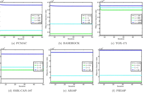
In the following subsections, we first evaluate con-vergence rate of the proposed JGSC on all datasets, for evaluating the efficiency of our proposed optimization Algorithm 2, in terms of the objective function value in each iteration. Then we test the parameters’ sensitiv-ity of the proposed JGSC according to the variation of the parameters, such as λ andα in Eq.3.4, aiming at achieving the best performance of the proposed JGSC. Finally, we compare JGSC with the comparison algo-rithms in terms of average classification accuracy (ACA for short).
Given a data pointxi, let yiand ˆyibe the derived
labels via a classification algorithm and the true label respectively. The ACA is defined as follows:
ACA=
Pn
i=1δ(yi,yˆi)
n (5.17)
where n is the sample size, δ(x, y) = 1 ifx =y, and δ(x, y) = 0, otherwise. The larger the performance on ACA is, the better the method.
5.2 Convergence rate In this subsection, we want to know the convergence rate of Algorithm 2, so we report some of the results in Fig.3 due to lack of space. Fig.3 shows the results of the objective function value while fixing the value ofαand varyingλ.
We can observe in Fig.3: 1) the objective function value rapidly decreases at the first few iterations; and 2) the objective function value becomes stable after about 30 iterations (or even less than 20 iterations in
10 20 30 40 50 0 2 4 6 8 10 12 14x 10 4 Iteration
Objective function value
λ = 50 λ = 100 λ = 500 λ = 1200 (a) PCMAC 10 20 30 40 50 0 0.5 1 1.5 2 2.5 3 3.5 4 4.5x 10 5 Iteration
Objective function value
λ = 0.01 λ = 1 λ = 10 λ = 50 (b) BASEHOCK 10 20 30 40 50 2 2.5 3 3.5 4 4.5 5 5.5 6 6.5x 10 10 Iteration
Objective function value
λ = 100 λ = 800 λ = 1200 λ = 1800 (c) TOX-171 10 20 30 40 50 0 0.5 1 1.5 2 2.5x 10 5 Iteration
Objective function value
λ = 0.5 λ = 2 λ = 5 λ = 10 (d) SMK-CAN-187 10 20 30 40 50 0 2 4 6 8 10 12x 10 7 Iteration
Objective function value
λ = 0.01 λ = 0.1 λ = 1 λ = 10 (e) AR10P 10 20 30 40 50 0 1 2 3 4 5x 10 7 Iteration
Objective function value
λ = 0.01 λ = 0.1 λ = 1 λ = 10
(f) PIE10P
Figure 3: An illustration on convergence rate of Algorithm 2 for solving the proposed objective function with fixedα.
many cases) on all datasets. This confirms that the fast convergence rate of Algorithm 2 to solve the proposed optimization problem in Eq.3.4. Similar results are observed for otherαandλvalues.
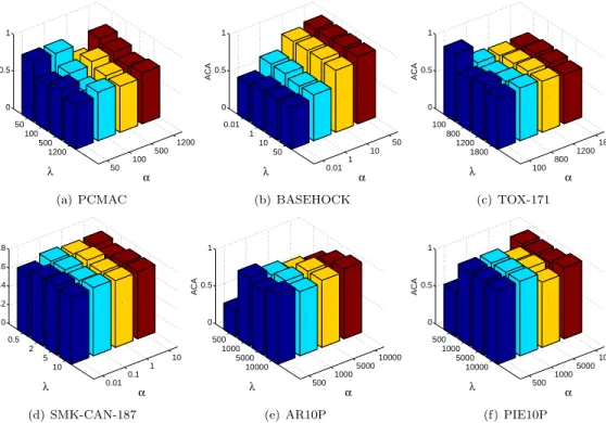
5.3 Parameters’ sensitivity In this subsection we study the classification performance of JGSC with re-spect to the variations of different parameters’ settings, i.e.,λandαin Eq.3.4. Due to the page limit, we only report the results on the case with 50% dimensionality left from the original dimensionality. The other cases have similar results. The experimental results are pre-sented in Fig. 4.
As can be seen in Fig. 4, JGSC is sensitive to the parameter setting. According to the experimental results, the average maximal improvement of the best results to the worst ones in the six datasets varies from 17.76% to 85.38%. Moreover, to obtain the best classification performance, different datasets need to set parameters differently.
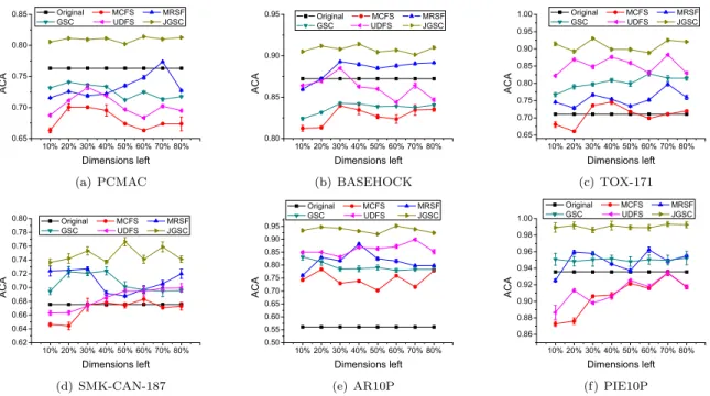
5.4 Classification results by all algorithms The classification performance ACA by all algorithms is presented in Fig. 5. The horizontal axis represents the number of the dimensions left after performing feature
selection, and the values vary from 10% to 80%. The vertical axis describes the value of ACA.
According to Fig.5, we have the following observa-tions: 1) The proposed JGSC achieves the best perfor-mance. This is obviously because the proposed JGSC overcomes all three drawbacks of MCFS, but each of the rival algorithms only solves part of the problems. More-over, JGSC outperforms UDFS, which also considers two constraints (i.e., discriminative ability and mani-fold learning with theℓ2,1-norm regularizer) to perform
feature selection. 2) The results of “Original” are better than the results of some dimensionality reduction algo-rithms on some datasets. However, these dimensionality reduction algorithms are more efficient due to their sig-nificantly reduced dimensionality of the datasets. Thus it is crucial for conducting dimensionality reduction on high-dimensional data. This is consistent with the con-clusion in [2, 4, 13]. 3) Although both MCFS and GSC lead to the element sparsity, the classification perfor-mance of MCFS is worse than GSC. This occurs because GSC simultaneously performs manifold learning and re-gression, but MCFS sequentially performs them. This demonstrates that simultaneously performing manifold learning and regression is better. 4) MRSF outperforms MCFS. That is because MRSF has more advantages
50 100 500 1200 50 100 500 1200 0 0.5 1 α λ ACA (a) PCMAC 0.01 1 10 50 0.01 1 10 50 0 0.5 1 α λ ACA (b) BASEHOCK 100 800 1200 1800 100 800 1200 1800 0 0.5 1 α λ ACA (c) TOX-171 0.010.1 1 10 0.5 2 5 10 0 0.2 0.4 0.6 0.8 α λ ACA (d) SMK-CAN-187 500 1000 5000 10000 500 1000 5000 10000 0 0.5 1 α λ ACA (e) AR10P 500 1000 5000 10000 500 1000 5000 10000 0 0.5 1 α λ ACA (f) PIE10P
Figure 4: ACA results on different datasets with different parameters.
than MCFS by replacing the ℓ1-norm regularizer with
theℓ2,1-norm regularizer, such as considering the
corre-lations among the spectral features and leading to the row sparsity. 5) The literatures (e.g., [2, 13]) have shown that their methods (e.g., UDFS and MCFS) outperform the popular methods, such as LPP [5], LScore [4], so we can make the conclusion that JGSC also outperforms LPP and LScore.
6 Conclusion
In this paper, we propose a novel feature selection method to deal with high-dimensional data. Moreover, we have shown that our method theoretically makes the proposed objective function converge to its global optimum. Furthermore, the experimental results have shown the effectiveness of the proposed method. In the future we will extend the proposed method into its kernel edition to deal with more complex cases, such as datasets with limited data points.
7 Acknowledgements
This research has been supported by the US Na-tional Science Foundation (NSF) under grant CCF-0905337; the Australian Research Council (ARC) under large grant DP0985456; the Nature Science
Foundation (NSF) of China under grants 61170131 and 61263035; the China 863 Program under grant 2012AA011005; the China 973 Program under grant 2013CB329404; the Guangxi Natural Science Foun-dation under grant 2012GXNSFGA060004; and the Guangxi “Bagui” Teams for Innovation and Research.
References
[1] Mikhail Belkin, Partha Niyogi, and Vikas Sindhwani. Manifold regularization: A geometric framework for
learning from labeled and unlabeled examples. Journal
of Machine Learning Research, 7:2399–2434, 2006. [2] Deng Cai, Chiyuan Zhang, and Xiaofei He.
Unsuper-vised feature selection for multi-cluster data. InACM
Special Interest Group on Knowledge Discovery and Data Mining, pages 333–342, 2010.
[3] Shenghua Gao, Ivor Wai-Hung Tsang, Liang-Tien Chia, and Peilin Zhao. Local features are not lonely - laplacian sparse coding for image classification. In
IEEE Conference on Computer Vision and Pattern Recognition, pages 3555–3561, 2010.
[4] Xiaofei He, Deng Cai, and Partha Niyogi. Laplacian
score for feature selection. In Neural Information
Processing Systems, pages 1–8, 2005.
[5] Xiaofei He and Partha Niyogi. Locality preserving
10%20%30%40%50%60%70%80% 0.65 0.70 0.75 0.80 0.85 A C A Dimensions left Original MCFS MRSF GSC UDFS JGSC (a) PCMAC 10%20%30%40%50%60%70%80% 0.80 0.85 0.90 0.95 A C A Dimensions left Original MCFS MRSF GSC UDFS JGSC (b) BASEHOCK 10%20%30%40%50%60%70%80% 0.65 0.70 0.75 0.80 0.85 0.90 0.95 1.00 A C A Dimensions left Original MCFS MRSF GSC UDFS JGSC (c) TOX-171 10%20%30%40%50%60%70%80% 0.62 0.64 0.66 0.68 0.70 0.72 0.74 0.76 0.78 0.80 A C A Dimensions left Original MCFS MRSF GSC UDFS JGSC (d) SMK-CAN-187 10%20%30%40%50%60%70%80% 0.50 0.55 0.60 0.65 0.70 0.75 0.80 0.85 0.90 0.95 A C A Dimensions left Original MCFS MRSF GSC UDFS JGSC (e) AR10P 10%20%30%40%50%60%70%80% 0.86 0.88 0.90 0.92 0.94 0.96 0.98 1.00 A C A Dimensions left Original MCFS MRSF GSC UDFS JGSC (f) PIE10P
Figure 5: The results of ACA on various parameters’ settings on different datasets. Note that, the range shown at the curves represents the performance standard deviation.
jections. In Neural Information Processing Systems,
pages 197–204, 2003.
[6] Sotiris Kotsiantis. Feature selection for machine learn-ing classification problems: a recent overview. Artifi-cial Intelligence Review, pages 1–20, 2011.
[7] Honglak Lee, Rajat Raina, Alex Teichman, and An-drew Y. Ng. Exponential family sparse coding with
applications to self-taught learning. In International
Joint Conference on Artificial Intelligence, pages 1113– 1119, 2009.
[8] Julien Mairal, Francis Bach, Jean Ponce, and
Guillermo Sapiro. Online learning for matrix
factoriza-tion and sparse coding. Journal of Machine Learning
Research, 11:19–60, 2010.
[9] Sebasti´an Maldonado and Richard Weber. A wrapper
method for feature selection using support vector
ma-chines. Information Science Journal, 179:2208–2217,
2009.
[10] Feiping Nie, Heng Huang, Xiao Cai, and Chris Ding. Efficient and robust feature selection via joint
l2,1-norms minimization. InNeural Information Processing
Systems, pages 1813–1821, 2010.
[11] Rajat Raina, Alexis Battle, Honglak Lee, Benjamin
Packer, and Andrew Y. Ng. Self-taught learning:
transfer learning from unlabeled data. InInternational Conference on Machine Learning, pages 759–766, 2007. [12] Zenglin Xu, Rong Jin, Jieping Ye, and Michael R. Lyu. Discriminative semi-supervised feature selection
via manifold regularization. IEEE Transactions on
Neural Networks, 21(7):1033–1047, 2010.
[13] Yi Yang, Heng Tao Shen, Zhigang Ma, Zi Huang, and Xiaofang Zhou. ℓ2,1-norm regularized discriminative
feature selection for unsupervised learning. In
Inter-national Joint Conferences on Artificial Intelligence, pages 1589–1594, 2011.
[14] Ming Yuan and Yi Lin. Model selection and estimation
in regression with grouped variables. Journal of the
Royal Statistical Society, Series B, 68:49–67, 2006.
[15] Zheng Zhao, Lei Wang, and Huang Liu. Efficient
spectral feature selection with minimum redundancy. InAAAI Conference on Artificial Intelligence, 2010. [16] Miao Zheng, Jiajun Bu, Chun Chen, Can Wang,
Lijun Zhang, Guang Qiu, and Deng Cai. Graph
regularized sparse coding for image representation.
IEEE Transactions on Image Processing, 20(5):1327 – 1336, 2011.
[17] Xiaofeng Zhu, Zi Huang, Heng Tao Shen, Jian Cheng,
and Changsheng Xu. Dimensionality reduction by
mixed kernel canonical correlation analysis. Pattern
Recognition, 45(8):3003–3016, 2012.
[18] Xiaofeng Zhu, Zi Huang, Yang Yang, Heng Tao Shen, Changsheng Xu, and Jiebo Luo. Self-taught dimen-sionality reduction on the high-dimensional small-sized
data. Pattern Recognition, 46(1):215–229, 2013.