Classification Rules for Data
Characterization
Achilleas Tziatzios
A thesis submitted in partial fulfilment of the requirements
for the degree of Doctor of Philosophy
in Computer Science
School of Computer Science & Informatics
Cardiff University
This work has not been submitted in substance for any other degree or award at this or any other university or place of learning, nor is being submitted concur-rently in candidature for any degree or other award.
Signed (candidate) Date
STATEMENT 1
This thesis is being submitted in partial fulfillment of the requirements for the degree of PhD.
Signed (candidate) Date
STATEMENT 2
This thesis is the result of my own independent work/investigation, except where otherwise stated. Other sources are acknowledged by explicit references. The views expressed are my own.
Signed (candidate) Date
STATEMENT 3
I hereby give consent for my thesis, if accepted, to be available for photocopying and for inter-library loan, and for the title and summary to be made available to outside organisations.
Signed (candidate) Date
STATEMENT 4: PREVIOUSLY APPROVED BAR ON ACCESS
I hereby give consent for my thesis, if accepted, to be available for photocopy-ing and for inter-library loans after expiry of a bar on access previously approved by the Academic Standards & Quality Committee.
“To my family and close friends for never quite losing their patience with me on this.”
Advances in data gathering have led to the creation of very large collections across different fields like industrial site sensor measurements or the account statuses of a financial institution’s clients. The ability to learn classification rules, rules that associate specific attribute values with a specific class label, from this data is important and useful in a range of applications.
While many methods to facilitate this task have been proposed, existing work has focused on categorical datasets and very few solutions that can derive classification rules of associated continuous ranges (numerical intervals) have been developed. Furthermore, these solutions have solely relied in classification performance as a means of evaluation and therefore focus on the mining of mutually exclusive classification rules and the correct prediction of the most dominant class values. As a result existing solutions demonstrate only limited utility when applied for data characterization tasks.
This thesis proposes a method that derives range-based classification rules from numerical data inspired by classification association rule mining. The presented method searches for associated numerical ranges that have a class value as their consequent and meet a set of user defined criteria. A new interestingness mea-sure is proposed for evaluating the density of range-based rules and four heuristic based approaches are presented for targeting different sets of rules. Extensive experiments demonstrate the effectiveness of the new algorithm for classification tasks when compared to existing solutions and its utility as a solution for data characterization.
This work would not have been possible without the support of Dow Corning Corporation and the people involved in the PR.O.B.E. project. I owe deep debt of gratitude to my supervisor Dr. Jianhua Shao for his guidance and mentorship during my years of study.
I would like to thank my friends and colleagues at the School of Computer Science and Informatics for their help and encouragement. More importantly I am very grateful to Dr. Gregorios Loukides for our long standing friendship and collabo-ration.
Finally, I thank my family for their continuous support and the entire EWOK team at Companies House for their understanding and encouragement during my writing up stage.
1 Introduction 1
1.1 Classification Rule Mining . . . 2
1.1.1 Mining of Continuous Data Ranges . . . 4
1.2 Research Challenges . . . 5
1.2.1 The Data Characterization Challenge . . . 6
1.3 Research Contributions . . . 7
1.4 Thesis Organization . . . 8
2 Background Work 10 2.1 Range-Based Classification Rule Mining: Concepts and Algorithms 10 2.2 Discretization . . . 11 2.2.1 Unsupervised Discretization . . . 13 2.2.2 Supervised Discretization . . . 14 2.3 Range-based Associations . . . 16 2.4 Associative Classification . . . 19 2.5 Rule Evaluation . . . 20 2.5.1 Objective Measures . . . 21 2.5.2 Subjective Measures . . . 24
2.6 Other Related Methods . . . 25
2.6.1 Performance Optimization Methods . . . 26
2.8 Summary . . . 27
3 Range-Based Classification Rule Mining 29 3.1 Preliminaries . . . 30 3.2 Interestingness Measures . . . 31 3.2.1 Support-Confidence . . . 32 3.2.2 Density . . . 33 3.3 Methodology . . . 34 3.3.1 Minimum Requirements . . . 34
3.3.2 Consequent bounded rules . . . 35
3.3.3 Finding Consequent Bounded Rules . . . 38
3.3.4 Generating Largest 1-ranges . . . 39
3.3.5 Generating Largest (i+ 1)-ranges . . . 42
3.3.6 LR Structure . . . 43
3.3.7 Splitting Largest Ranges Into Consequent Bounded Rules . . 44
3.4 Summary . . . 45
4 CARM Algorithm 47 4.1 Heuristics . . . 47
4.1.1 Maximum Support Heuristic . . . 48
4.1.2 Maximum Confidence Heuristic . . . 52
4.1.3 Maximum Gain Heuristic . . . 56
4.1.4 All Confident Heuristic . . . 59
4.2 Summary . . . 62
5 Evaluation of Range-Based Classification Rule Mining 63 5.1 Data Description . . . 63
5.2 Classification Experiments . . . 64
5.2.2 Prediction Accuracy . . . 84
5.3 Characterization . . . 95
5.3.1 Differences Between Characterization And Classification . . 96
5.3.2 Characterization Evaluation . . . 96
5.4 Summary . . . 105
6 Conclusions and Future Work 106 6.1 Conclusions . . . 106
6.2 Applications . . . 108
6.3 Future work . . . 109
6.3.1 Modifications . . . 110
1.1 Classification model built by Naive Bayes for the iris dataset. . . 3
1.2 Classification rules model built by RIPPER for the iris dataset. . . 3
1.3 Mining data areas of interest. . . 7
2.1 The research space of association mining. . . 11
2.2 The research space of discretization. . . 13
2.3 Single optimal region compared to multiple admissible regions. . . . 18
2.4 Associative classification mining by filtering of association rules. . . 19
3.1 Consequent bounded rules . . . 36
3.2 LR structure for storing candidate rules. . . 42
3.3 LR structure for storing candidate rules. . . 43
4.1 Graphic representation of a range split. . . 47
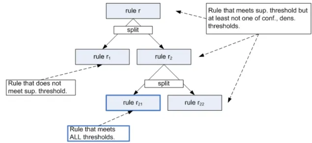
4.2 Tree generated by maximum support splits. . . 52
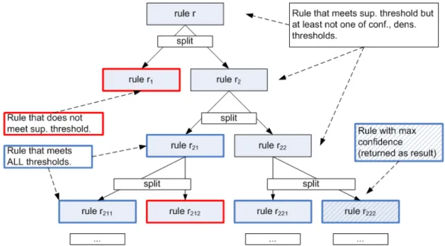
4.3 Tree generated by maximum confidence splits. . . 56
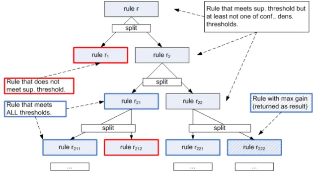
4.4 Tree generated by maximum gain splits. . . 59
4.5 Tree generated by maximum gain splits. . . 61
5.1 Density effect on prediction accuracy of breast cancer data. . . 66
5.2 Density effect on prediction accuracy of ecoli data. . . 68
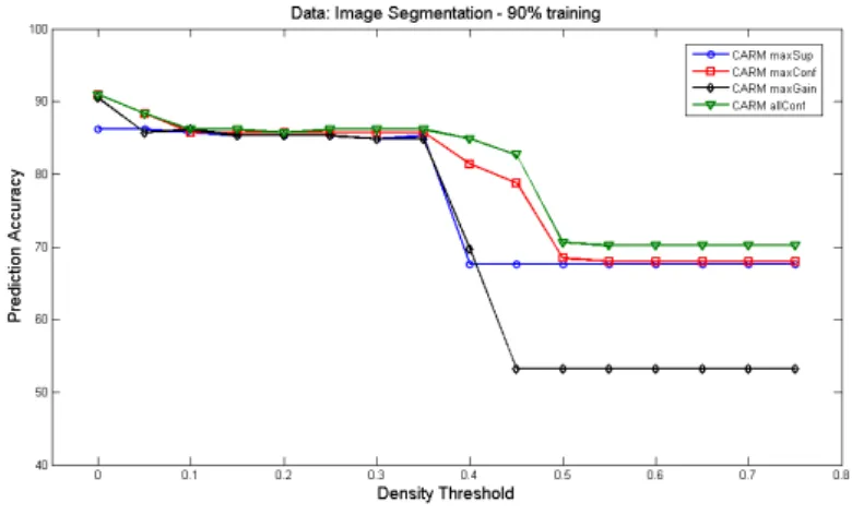
5.4 Density effect on prediction accuracy of image segmentation data. . 72
5.5 Density effect on prediction accuracy of iris data. . . 73
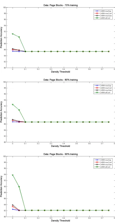
5.6 Density effect on prediction accuracy of page blocks data. . . 75
5.7 Density effect on prediction accuracy of waveform data. . . 77
5.9 Density effect on prediction accuracy of wine data. . . 79
5.10 Density effect on prediction accuracy of red wine quality data. . . . 80
5.11 Density effect on prediction accuracy of white wine quality data. . . 82
5.12 Density effect on prediction accuracy of yeast data. . . 84
5.13 Prediction accuracy comparison for the breast cancer dataset . . . . 86
5.14 Prediction accuracy comparison for the ecoli dataset . . . 87
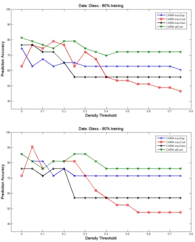
5.15 Prediction accuracy comparison for the glass dataset . . . 88
5.16 Prediction accuracy comparison for the image segmentation dataset 88 5.17 Prediction accuracy comparison for the iris dataset . . . 89
5.18 Prediction accuracy comparison for the page blocks dataset . . . 90
5.19 Prediction accuracy comparison for the waveform dataset . . . 90
5.20 Prediction accuracy comparison for the wine dataset . . . 91
5.21 Prediction accuracy comparison for the wine quality red dataset . . 92
5.22 Prediction accuracy comparison for the wine quality white dataset . 92 5.23 Prediction accuracy comparison for the yeast dataset . . . 93
5.24 Box plot for prediction summary results. . . 95
5.25 A model consisting of non overlapping rules . . . 97
5.26 A model consisting of several representations using overlapping rules 98 5.27 Prediction accuracy consistency for breast cancer data. . . 99
5.28 Prediction accuracy consistency for ecoli data. . . 100
5.29 Prediction accuracy consistency for glass data. . . 100
5.30 Box plot for density cohesion of 10 most confident rules results. . . 103
1.1 Description of the iris dataset. The possible class values arehiris−
setosa, iris−versicolor, iris−virginicai. . . 2
2.1 Bank clients database. . . 12
2.2 Bank clients database with account balance discretized. . . 12
2.3 An equi-depth discretization of Checking Account balanceand Savings Account balance into 10 bins. . . 17
3.1 Bank clients and issued loans data. . . 30
3.2 Table 3.1 after sorting values per attribute. . . 40
3.3 LR1 ranges for the attributes of Table 3.1 . . . 41
4.1 The original ruler. . . 51
4.2 The resulting rulesr10 : [v6, v10]A1∧[u4, u7]A2 ⇒ckandr20 : [v14, v9]A1∧ [u4, u7]A2 ⇒ck. . . 51
4.3 The original ruler. . . 55
4.4 The resulting rulesr10 : [v6, v9]A1∧[u4, u16]A2 ⇒ckandr20 : [v6, v9]A1∧ [u11, u7]A2 ⇒ck. . . 55
5.1 Datasets . . . 64
5.2 A possible voting table . . . 86
5.4 ANOVA table for prediction summary results. . . 95 5.5 An example of a voting table . . . 98 5.6 Median density cohesion for the 10 most confident rules. . . 102 5.7 ANOVA table for density cohesion of 10 most confident rules results.103 5.8 Median density cohesion for the 10 most supported rules. . . 104 5.9 ANOVA table for density cohesion of 10 most supported rules results.104
Introduction
Recent advances in data generation and collection have led to the production of massive data sets in commercial as well as scientific areas. Examples of such data collections vary from data warehouses storing business information, biological databases storing increasing quantities of DNA information for all known organ-isms and the use of telescopes to collect high-resolution images of space [10, 57]. The speed at which data is gathered has far exceeded the rate at which it is being analysed.
Data mining is a field that grew for the purpose of using the information contained in these data collections and out of the limitations of existing techniques to handle the ever growing size as well as the evolving types of data. Data Mining, often referred to as Knowledge Discovery in Databases (KDD), refers to the nontriv-ial extraction of implicit, previously unknown and potentnontriv-ially useful information from data in databases. While data mining and knowledge discovery in databases (or KDD) are frequently treated as synonyms, data mining is actually part of the knowledge discovery process. Business applications range from predictive mod-els for management decision making, to pattern extraction for customer services personalisation as well as optimisation of profit margins.
Since the goal was to meet the new challenges, data mining methodologies are strongly connected, and often build upon existing areas of data analysis. Just like with any rapid growing research field, data mining methods have evolved as different research challenges and applications, stemming from different areas, have emerged. A significant portion of research work has actually focused on defining the field and/or its relationship to existing fields [19, 36, 47, 53, 69, 93].
1.1
Classification Rule Mining
The problem of discovering knowledge in data is complex to define. The three main areas of data mining tasks consist of classification, association analysis and
clustering [36, 52, 106]. Classification is the task of constructing a model from data for a target variable, referred to as the class label. Association analysis is the discovery of patterns of strongly associated features in the given data whereas clustering seeks to find groups of closely related data values so that data that are clustered together are more similar than with the remaining data.
In certain cases, however, the desired result of the data mining process may not be as discrete as described and the designed solution is a combination of more than one of the above tasks. An example of this is the area that this thesis is focused on, associative classification rule mining [74], where the goal is mining associations of data variables that are also associated with a specific class label. The following examples show the difference between a typical classification algorithm likeNaive Bayes [61] in Figure 1.1 and an association rule mining algorithm likeRIPPER[22] when used to mine associations only for a specific target variable in Figure 1.2. The data used are that of the well known iris dataset which is described in Table 1.1.
Attribute sepal length sepal width petal length petal width class
Type numeric numeric numeric numeric categorical
Table 1.1: Description of the iris dataset. The possible class values are hiris−
setosa, iris−versicolor, iris−virginicai.
Note in Figure 1.2 that the RIPPER algorithm generates a complete model and not independent rules. In order for each rule to be a complete classification rule its predicate needs to include the negation of any preceding rules in the model. A typical classification solution, however as in Figure 1.1, presents its results in a single model.
Figure 1.1: Classification model built by Naive Bayes for the iris dataset.
1.1.1
Mining of Continuous Data Ranges
Another important distinction between data mining tasks is based on the type of data mined. The type of each attribute is indicative of its underlying properties and therefore an important aspect of a data mining method is the type of data it is designed to mine. The iris data used in the example consists of numerical, more specifically continuous, data attributes. In real world applications this is expected to be the case in the majority of tasks since real world data collections often contain real numbers. However existing work in the area of classification rule mining has focused primarily on mining data of a categorical nature. Applying these solutions on continuous values requires discretization of the given data. For example, a possible discretization of the petal length attribute of the iris dataset would transform the continuous attribute into a categorical one with three possible values h(−∞,2.45],(2.45,4.75],(4.75,+∞)i so that a method designed for a categorical attribute can be applied. These solutions may be applicable on continuous data that have been transformed to categorical but determining a good way of transforming real values to categorical ones constitutes another research problem in itself.
Not all existing solutions require continuous data to be discretized. Algorithms like RIPPER, in the given example, choose the best value at which to split a con-tinuous attribute so that one of the resulting ranges maximizes a target measure. In some cases a rule may actually contain a range of continuous values like in Fig-ure 1.2 the rule (petallength ≥ 3.3) and (petalwidth ≤ 1.6) and (petallength ≤
4.9)⇒class=Iris-versicolor includes the rangepetallength∈[3.3,4.9] but this is the result of two binary splits that first selected the petal-length values that were ≥ 3.3 and amongst the values that met the requirements (petallength ≥
3.3) and (petalwidth ≤ 1.6) another binary split was performed at petal length 4.9. Furthermore, any relation of the form attribute ≤ v may be interpreted as a range attribute ∈ (−∞, v] where −∞ may also be replaced with the vmin of attribute. Regardless of representation, however these ranges are the result of binary splits. This thesis presents a solution that for all continuous attributes attempts to mine multiple continuous ranges directly from the real(R) values of an attribute.
1.2
Research Challenges
The data mining area has been developed in order to address limitations of tra-ditional data analysis. However, the fast evolution of modern data collections continues to pose a plethora of important research challenges in the development of data mining solutions. This section presents an overview of these challenges and discusses how they relate to the solution presented in this thesis.
• Scalability: Advances in data generation and collection have led to datasets of a very large size becoming more and more common. Therefore, modern data mining solutions need to be scalable in order to handle these datasets. The development of scalable algorithms may require the implementation of novel, efficient data structures, an efficient reduction of the problem space via sampling techniques or the development of a solution that may be executed in parallel threads. The area of parallel executed solutions is evolving fast and is expected to address many of the limitations of current data mining solutions [26, 62]. Typically, scalability refers to the number of records(rows) in a dataset but modern collections may include thousands of attributes for each record, presenting researchers with the added challenge ofhigh dimen-sional data for algorithms whose complexity increases with the number of attributes.
• Heterogeneous and Complex Data: Traditional data collections con-sist of homogeneous data therefore simplifying the analysis process. Due to the increasing number of areas where data mining is applied, however, new cases arise where heterogeneous attributes need to be mined. More impor-tantly, the inclusion of new types of complex data objects, in the forms of text data, genomes and even structured text(code) in the case of XML doc-uments requires the development of data mining solutions that incorporate the relations between the mined data values.
• Distributed data sources: In some cases the data are not located in a single central storage and possibly owned by many different legal entities. Therefore, mining the data as a single dataset incorporating all the infor-mation from individual sources poses an important challenge. Furthermore, the issue of data privacy is another challenge when the aforementioned data sources include sensitive information that may be used for the purpose of mining the data but cannot, under any circumstance, be related to
individ-uals in the resulting model.
• Non traditional analysis: The traditional statistical approach focuses mainly on the testing of hypotheses, rather than generating them from the data as modern data mining tasks attempt to achieve. In order to effectively discover knowledge in the data a data mining method needs to generate and test a large number of hypotheses/models. The main areas of data mining, as mentioned in Section 1.1, cover the traditional research problems but modern analysis has diversified itself due to the incorporation of non traditional data types as well as non traditional expectations from the results. Section 1.2.1 describes such a task that this thesis attempts to address.
1.2.1
The Data Characterization Challenge
In the example of Section 1.1 the expectation is the ability to effectively classify any future iris specimen into one of the given classes. However, as explained the nature of data mining has evolved and there are tasks that go beyond the scope of predictive modelling. Large historical data collections cannot always be modelled with sufficient accuracy, or due to the volume of the data it is possible that constructing a complete model of the data is not realistic. In these cases the desired data mining output is a set of hypotheses about specific data areas that can be tested and verified by domain experts in order to gain knowledge on the process.
Improving a process relies on a good understanding of it and the data used to monitor it. Causality is the relation between an event and a phenomenon, referred to as the effect [34], and in order to effectively comprehend a phenomenon and either replicate or avoid it is necessary to comprehend its underlying mechanisms. Consider the example of a high performance race car. Testing as well as racing provides a team of engineers with a large volume of data regarding the car’s performance. Due to time limitations as well as the lack of established knowledge for the novel, cutting edge technologies employed it is not realistic to develop a complete model of the car’s behavior and consequently the optimal performance. The only realistic option is to identify positive scenarios, as data areas, and study them in order to gain knowledge on the conditions that can potentially improve overall performance. Alternatively, improvement may be achieved by identifying negative, or undesirable scenarios and avoiding the conditions that constitute the
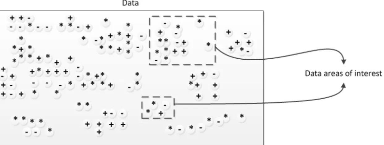
underlying causes. Note how we refer to improved, not optimal, performance as there is no such guarantee in this case. Figure 1.3 graphically represents the extraction of such data areas.
Figure 1.3: Mining data areas of interest.
In the given figure the data samples have been classified in three different classes
h+,−,∗iforhpositive, negative, averageiperformance respectively. In the case of mining continuous attributes these areas are represented as classification rules of associated numerical ranges.
The distinctive difference in data characterization is that the value of the result is not based on its effectiveness of predicting new, previously unseen, data but improving the understanding of the existing dataset. In the classification context the user asks for a data model that can be applied to a new, unlabeled dataset, in characterization the desired output needs to be applicable to the training data and provide information about the original dataset. This is because in characterization we refer to users that aim to improve an underlying process and not only predict future output.
1.3
Research Contributions
Mining a single optimal numerical range with regards to an interest measure can be mapped to the max-sum problem. For a single attribute a solution using dy-namic programming can be computed in O(N) [9]. When the desired optimal range is over two numerical attributes then the problem isNP-hard [41, 42]. The problem of mining multiple continuous ranges that optimize a given criterion can
be mapped to thesubset sum problem that is NP-complete [23]. This thesis’ con-tribution is a scalable, effective solution that employs a heuristics-based approach. The presented methodology addresses datasets of continuous attributes and mines continuous ranges without any form of pre-processing of the data.
The primary contribution, however, of the developed algorithm is to the non traditional analysis challenge, focusing on addressing the data characterization problem. The solution described in the following chapters mines multiple rules of associated numerical ranges from continuous attributes that can be used in a data characterization scenario. Due to the nature of the problem the algorithm developed is using user-set thresholds, for the interest measures employed, as input. The presented solution is flexible, allowing for users to tune the input thresholds to different values that describe the targeted knowledge.
Extensive experiments demonstrate the effectiveness of the presented solution as a classification algorithm as well as in the area of data characterization. Further-more, the distinctive differences in evaluating prediction accuracy and characteri-zation effectiveness are described and employed in a comparison that demonstrates the advantages of the developed solution.
1.4
Thesis Organization
The remaining chapters of this thesis are structured as follows.Chapter 2 reviews work in the related associative classification literature. Research on mining contin-uous datasets as well as related rule association methods are analysed. Further-more, an overview of existing interestingness measures for mining classification rules is presented as well as a review of existing solutions that have or could potentially address the data characterization problem.
Chapter 3 introduces important definitions and key concepts for the presented methodology. Furthermore, the concept of bounded ranges is presented as a method for reducing search space. The general algorithm is described for identi-fying ranges from the continuous attributes and incrementally building them into range-based rule candidates. Chapter 3 includes the concept and formal definition of a novel interestingness measure designed specifically for continuous numerical ranges. Also, the usage of a custom data structure for storing the candidates is given as well as a presentation of the concept of splitting candidates into range-based rules.
Following the general description, Chapter 4 presents four(4) different criteria for splitting rule candidate rules into the resulting range-based classification rules. The significance and exact methodology for each heuristic are explained along with the strengths and weaknesses of each method.
Chapter 5 presents an evaluation of the developed solution compared to existing algorithms. A comparative study is given for how the newly introduced interest measure affects classification outcome on a series of datasets. The experimental results for predicting unlabeled data using the described methods are provided and compared against established rule mining solutions implemented in Weka
[51]. Chapter 5 also includes a series of experiments based on key aspects of the characterization problem that demonstrate how the presented solution addresses these tasks.
Finally, Chapter 6 concludes the thesis and discusses future directions for extend-ing the presented work.
Background Work
In this chapter, we present an overview of the literature on range-based classifica-tion rule mining and discuss how existing techniques on related problems compare to ours.
2.1
Range-Based Classification Rule Mining:
Con-cepts and Algorithms
In order to classify related work in the area of associative classification we use the three main aspects of each approach as described below.
• The nature of the input data.
• The approach for mining the rules.
• The measures used for evaluating the rules.
The nature of the input data refers to the different types of datasets and their char-acteristics. Two different types of data are categorical and numerical/continuous
whereas an example of data with special characteristics are time series data due to the sequential relationship between data values. This chapter discusses methods designed to handle different data types but focuses primarily on methods capable of mining continuous data. The mining approach refers to the method used for generating the rules whereas the evaluation measures concern the different criteria employed in each case for determining each rule’s importance which we refer to as
The problem of deriving range-based classification rules can be viewed as a problem of supervised discretization which we analyze in Section 2.2. In Section 2.3 we present existing work on mining range-based association rules whereas in section 2.4 we examine work in the area ofassociative classification which covers methods that incorporate characteristics of both association rule mining and classification.
A more detailed overview of the research space of associative classification can be seen in Figure 2.1.
Figure 2.1: The research space of association mining.
Other approaches related to association mining that do not address the associative classification problem, and are therefore not so closely related to our work are reviewed in Section 2.6.
2.2
Discretization
One way to address the problem of mining continuous data is by discretizing the continuous attributes. Discretization is the process of transforming a continuous attribute into a categorical one [67, 77]. A special form of discretization is bina-rization when continuous and categorical attributes are transformed into one or more binary attributes.
Consider the database in Table 2.1 which represents a bank’s clients, their ac-counts’ balance and other useful information. The table attributes Checking Ac-count and Savings Account represent continuous features and could all be dis-cretized. In Table 2.2 you can see the database after the attributes Checking Account and Savings Account have been discretized.
In the aforementioned example a simplemanual method of discretization is shown in order to demonstrate the differences with Table 2.1. The hypothesis, in this case, is that the organization holding the data chooses to group clients in pre-specified ranges because, for example, it is believed that all clients with a checking account
ClientID Checking Account Savings Account Loan C1 2003.15 2000.0 long term C2 0.0 100.3 short term C3 56087.5 125000.0 -C4 127.3 0.45 long term C5 −345.2 5250.5 -C6 11023.04 0.0 short term C7 19873.6 22467.4 long term C8 4187.1 0.0 -C9 4850.36 445.2 short term C10 8220.4 3250.12 long term
Table 2.1: Bank clients database.
ClientID Checking Account Savings Account Loan
C1 (2000,5000] (1000,5000] long term C2 [0,1000] [0,1000] short term C3 (50000,100000] (100000,250000] -C4 [0,1000] [0,1000] long term C5 [−1000,0) (5000,20000] -C6 (5000,20000] [0,1000] short term C7 (5000,20000] (20000,50000] long term C8 (2000,5000] [0,1000] -C9 (2000,5000] [0,1000] short term C10 (5000,20000] (1000,5000] long term
Table 2.2: Bank clients database with account balance discretized.
balance in the range (50000,100000] have the same characteristics. Curved brack-ets are used when the corresponding value is not included in the range whereas squared brackets are used for values that are included in the range. For example, a value of 50000 is not included in the range (50000,100000] but 100000 is. In certain cases, discretization is a potential inefficient bottleneck, since the number of possible discretizations is exponential to the number of interval threshold can-didates within the data domain [32]. There have been attempts to address the difficulty of choosing an appropriate discretization method given a specific data set [17, 29].
Data can be supervised or unsupervised depending on whether it contains class information. Consequently, supervised discretization uses class information while
unsupervised discretization does not. Unsupervised discretization can be seen in early methods that discretize data in bins of eitherequal-width orequal-frequency. This approach does not produce good results in cases where the distribution of
the continuous attribute is not uniform and in the presence of outliers that af-fect the resulting ranges [16]. Supervised discretization methods were introduced where a class attribute is present to find the proper intervals caused by cut-points. Different methods use the class information for finding meaningful intervals in con-tinuous attributes. Supervised and unsupervised discretization have their different uses although the application of supervised discretization requires the presence of a class attribute. Furthermore, the application of an unsupervised discretization method requires a separate step of mining rules from the discretized data which is why we focus, primarily, on supervised classification. Discretization methods can also be classified based on whether they employ a top-down approach or bottom-up. Top-down methods start with the full range of a continuous attribute and attempt to gradually split it in smaller ones as they progress. Bottom-up meth-ods start with single values and attempt to gradually build larger numerical ranges by gradually merging them. Because of this we also refer to top-down methods as split-based whereas we refer to bottom-up methods as merge-based. A repre-sentation of the classification space for a discretization method can be seen in 2.2.
Figure 2.2: The research space of discretization.
2.2.1
Unsupervised Discretization
Binning is the method of discretizing continuous attributes into a specified num-ber of bins of equal width or equal frequency. Regardless of which method is followed, the number of bins k needs to be given as input. Each bin represents a distinct discrete value, a numerical range. In equal-width, the continuous range of a feature is divided into intervals of equal-width, each interval constitutes a bin.
In equal-frequency, the same range is divided into intervals with an equal number of values placed in each bin.
One of the major advantages of either method is their simplicity but their effec-tiveness relies heavily on the selection of an appropriate k value. For example, when using equal-frequency binning, many occurrences of the same continuous value could cause the same value to be assigned into different bins. A solution would be a post-processing step that merges bins that contain the same value but that also disturbs the equal-frequency property. Another problem is data that contain outliers with extreme values that require the removal of these values prior to discretization. In most cases, equal-width binning and equal-frequency binning will not result in the same discretization [77].
2.2.2
Supervised Discretization
Unsupervised binning is meant to be applied on data sets with no class information available. However, there are supervised binning methods that address this issue. 1R [56] is a supervised discretization method that uses binning to divide a range of continuous values into a number of disjoint intervals and then uses the class labels to adjust the boundaries of each bin. The width of each bin is originally the same and must be specified before execution. Then each bin is assigned a class label based on which class label is associated with the majority of values in the given bin, let that class label beCm. Finally, the boundaries of each adjacent bin are checked and if there are any values that are also associated with Cm they are merged with the given bin. 1R is comparatively simple to unsupervised binning but does not require the number of bins to be pre-specified, it does however, require the definition of an initial width for each bin. Another way has been developed for improving equal-frequency by incorporating class information when merging adjacent bins, by using maximum marginal entropy [29]. In spite of their ability to include the additional information neither approach has been shown to have better results than unsupervised binning when used for the mining of classification rules [77].
A statistical measure often employed in supervised discretization is chi-square
χ2 by using the χ2 −test between an attribute and the classifier. Methods that
use this measure try to improve discretization accuracy by splitting intervals that do not meet this significance level and merging adjacent intervals of similar class frequency [65]. There is a top-down approach, ChiSplit, based onχ2 that searches
for the best split of an interval, by maximizing the chi-square criterion applied to the two sub-intervals adjacent to the splitting point and splits the interval if both sub-intervals differ statistically. Contrary to ChiSplit, ChiMerge [65] performs a local search and merges two intervals that are statistically similar. Other ap-proaches continue to merge intervals while the resulting interval is consistent [78] or have attempted to apply the same criterion on multiple attributes concurrently [110]. Instead of locally optimizingχ2 other approaches apply theχ2−teston the entire domain of the continuous attributes and continuously merge intervals while the confidence level decreases [11].
Another measure used to evaluate ranges is entropy. An entropy-based method detects discretization ranges based on the classifier’s entropy.Class information entropy is a measure of purity and it measures the amount of information which would be needed to specify to which class an instance belongs. It is a top-down method that recursively splits an attribute in ranges while a stopping criterion is satisfied (e.g. a total number of intervals). Recursive splits result in smaller ranges, with a smaller entropy so the stopping criterion is usually defined to guarantee a minimum number of supported instances. An approach proposed by Fayyad et al. examines the class entropy of the two ranges that would result by splitting at each midpoint between two values and selects the split point which minimizes entropy [35]. When the size of the resulting ranges does not meet theminimum description length (MDL)the process stops. It has been shown that optimal cut points must lie between tuples of different class values [35, 54], a property that we also use in our approach. Other approaches attempt to maximize mutual dependence between the ranges and the class label and can detect the best number of intervals to be used for the discretization [20]. In [50] the authors merge the individual continuous values in ranges of maximum goodness while trying to maintain the highest average-goodness. This results in an efficient discretization but does not guarantee any of the desired classification properties for the resulting ranges. Finally, CAIM [68] uses class-attribute interdependence in order to heuristically minimize the number of discretized ranges. The authors demonstrate that this approach can result in a very small number of intervals, however unlike discretization, in range-based classification a small number of ranges is not desired when there are class values of low support.
Unlike discretization algorithms that are developed for the pre-processing step of a data mining algorithm there are methods that are designed to alter the nu-merical intervals based on the performance of an induction algorithm [15, 108].
In some cases algorithms are developed to adapt the ranges so as to minimize
false-positives and false-negatives on a training data set [18, 81]. One important limitation, however, is the need for a predetermined number of intervals. In ad-dition to techniques that consider error-rate minimization there are methods that integrate a cost function to adapt the cost of each prediction error to specific prob-lems [60]. It has been shown that in order to determine the optimal discretization that maximizes class information one only has to check a small set of candidate data points, referred to as alternation points. However, failure to check one alter-nation point may lead to suboptimal ranges [31]. This idea, has been extended to develop very efficient top-down discretization solutions given an evaluation func-tion [32] by removing any potential split-points that are proven suboptimal, from the algorithms search space.
More recently, research in discretization has focused onadaptive discretization
approaches. Adaptive Discretization Intervals (ADI) is a bottom-up approach that can use several discretization algorithms at the same time which are evalu-ated to select the best one for the given problem and a given data set [6]. ADI has also been extended to use heuristic non-uniform discretization methods within the context of a genetic algorithm during the evolution process when a different discretization approach can be selected for each rule and attribute [7]. The con-cept of adaptive classification during the evolution process of a genetic algorithm has been researched extensively [27, 46]. A comparison of the most well-known approaches can be found in [5].
2.3
Range-based Associations
This section examines existing solutions that address the problem of mining range-based rules from continuous data.
One of the first approaches at mining association rules from a data set that in-cludes both continuous and categorical attributes was in [102]. The aforemen-tioned solution mines a set of association rules but requires an equi-depth parti-tioning(discretization) of the continuous attributes. Therefore, the desired ranges can only result from merging these partitions and the original problem is mapped to a boolean association rules problem. Table 2.3 demonstrates an example of equi-depth partitioning of Table 2.1, note that the number of bins used for the discretization do not have to be the same for every attribute.
ClientID Checking Account Savings Account Loan C1 [−1000,4708.75] [0,12500] long term C2 [−1000,4708.75] [0,12500] short term C3 (50378.75,56087.5] (112500,125000] -C4 [−1000,4708.75] [0,12500] long term C5 [−1000,4708.75] [0,12500] -C6 (10417.5,16126.25] [0,12500] short term C7 (16126.25,21835] (12500,25000] long term C8 [−1000,4708.75] [0,12500] -C9 (4708.75,10417.5] [0,12500] short term C10 (4708.75,10417.5] [0,12500] long term
Table 2.3: An equi-depth discretization of Checking Account balance and
Savings Account balance into 10 bins.
Given Table 2.3 and two associationsCheckingAc∈[−1000,4708.75]∧SavingsAc∈
[0,12500] and CheckingAc ∈(4708.75,10417.5]∧SavingsAc∈ [0,12500] we can merge them into one rule that the authors refer to as super-rule CheckingAc ∈
[−1000,10417.5]∧SavingsAc∈[0,12500]. As you can see from this example, this approach results in association rule mining where the produced ranges depend on the discretization criteria, therefore, experimentation is required for producing appropriate bins that will give good results introducing an important limitation to this methodology. The approach of discretizing continuous data into ranges as a preprocessing step is a very popular one. In [64] a method is presented for mapping pairs of attributes to a graph based on their mutual information (MI)
score. This method is based on the assumption that all interesting associations must have a high MI score and therefore must belong in the same clique in the graph. In some cases, however, researchers have presented the problem of mining associations from data that is already stored in the form of numerical ranges [30] which is essentially directly comparable to the aforementioned methods after the discretization phase.
Different approaches have been described for directly generating numerical ranges from the data. Given a numerical attribute and a categorical class label in [39] the authors present an approach to solving two different problems. Mining the range of the numerical attribute with the maximum support, given a confidence threshold and mining the corresponding range with the maximum confidence given a support threshold. Unlike previously described solutions, this approach includes user defined thresholds for support and confidence, although for separate prob-lems. Furthermore, it is only applicable to one attribute, or data sets of more
attributes that only contain a single continuous attribute. An extension of this was described in [41, 42] where the solutions presented mine optimal ranges from two continuous attributes with a boolean attribute as the consequent. By using dynamic programming the aforementioned solution is able to mine the numerical range of maximumgain, an interest measure described in more detail in 2.5.1, but the result is a single region of optimal gain. Therefore, the aforementioned ap-proach does not address the problem of mining all range-based classification rules even in the problem space of two continuous attributes. The difference between the desired output in a two-dimensional problem space is represented in Figure 2.3.
(a) Single region of optimal gain. (b) Multiple admissible ranges.
Figure 2.3: Single optimal region compared to multiple admissible regions.
The problem of mining a single optimal gain region has been extended to mining an approximation of thekoptimal gain regions, as the problem of mining thekregions of optimal gain is NP-hard, from a data set that contains both continuous and categorical attributes [14]. The proposed method still relied in a pre-processing step that places contiguous values with the same class label in the same bucket and was still limited to a total of two attributes excluding the class label. In [72] the authors also limit the problem space to two dimensions but take a different approach, they develop a method for mining the most dense ranges, that is the ranges with the most data points within the range, from the data. The concept of data density is, actually, of particular interest when dealing with continuous data ranges as we explain in Chapter 3. However, there is no evidence to support that density by itself is a sufficient evaluation measure.
Other approaches have considered mining range-based rules as an optimization problem and proposed solutions using a genetic algorithm. The mined rules are associations between numerical ranges of attributes and not classification rules. In [83] a solution is presented that uses an evolutionary algorithm based on a fitness function that improves the generated ranges between generations. This solution is able to mine overlapping ranges of high support but offers poor results
in term of confidence. Quantminer [97] is a genetic-based algorithm that delivers better results in terms of confidence and a reduced number of rules. The proposed solution is efficient but offers no guarantees that its solutions will meet certain thresholds.
2.4
Associative Classification
Classification rule mining and association rule mining are two popular data mining tasks with distinct differences. Classification rule mining aims to discover a small set of rules in the data to form an accurate classifier [92] whereas association rule mining aims to find all the rules that satisfy some predetermined constraints [4]. For association rule mining, the target of mining is not predetermined, while for classification rule mining the rule target can only be a specific attribute, the class. Both classification rule mining and association rule mining are useful to practical applications, therefore integrating the two tasks can be of great benefit. The integration is achieved by focusing on a special subset of association rules whose consequent is restricted to the class attribute. We refer to these rules as class association rules (CARs) [74]. There are researchers, however, that have expressed the opinion that due to the fact that associative classification techniques are often evaluated based on prediction effectiveness that it is, essentially, another form of classification [37]. However, even though prediction is often used to evaluate associative classification methods it is not the only method. Moreover, we view associative classification as a powerful method that is capable of addressing more problems than just classification, especially when applied in real world problems. An approach for mining associative classification rules from categorical data is presented in [107] that seems to perform well compared to existing solutions. Early approaches have also adopted a simple technique which relied on a two-step process of mining associations from the data and then ranking the resulting rules based on a selected evaluation measure. The top ranking rules were considered to be the resulting associative classification rules as demonstrated in Figure 2.4.
This category of methods relies heavily on the selected evaluation measure and produces variable results depending on the data set [63, 86]. In some cases heuris-tics are applied to actively reduce the number of generated rules making the mining algorithm more efficient [115]. Alternatively, other researchers have addressed the problem of associative classification as a problem of modeling the data using R-Trees based on the different class labels and then trimming the resulting models in order to avoid overfitting and reduce the number of rules [71]. These solutions prioritise classification performance and aim to increase data coverage with the fewest rules possible. Besides being applied on categorical data only, these algo-rithms avoid the mining of less general but more specific rules that may represent important data characteristics as discussed in Section 1.2.1.
One popular method that can be employed for mining range based classification rules is the C4.5 algorithm [92]. This is a partitioning based technique that only looks for the best halving of the domain with regards to a specific class. It has a quadratic time complexity for non numeric data that increases by a logarithmic factor when numerical attributes are processed. C4.5 is inefficient when dealing with strongly correlated numerical attributes. In order to improve this an approach has been proposed that given a numeric attribute and a boolean class attribute it can produce a more efficient branching for the given attribute [40]. Unlike the original C4.5 algorithm , in the latter solution the attribute values are pre-discretized in a user set number of ranges and the discrete ranges are merged in order to produce an optimal branching that minimizes total entropy. Although the described approach has proven to improve the size of the tree and can be extended to work with class labels of more than two discrete values (non boolean), its outcome relies on the user selecting an appropriate number of buckets for the discretization whereas its classification accuracy is not evaluated. Furthermore, the direct output of these algorithms is aDecision Tree (DT) that requires further processing in order to transform the results into range-based classification rules. Even with the additional post-processing, however, there is no guarantee that the resulting rules meet any specific requirements (e.g. user specified thresholds).
2.5
Rule Evaluation
In this section we present measures that have been used by the research commu-nity for the evaluation of classification rules, which we refer to as interestingness
measures. We include measures that have originally been developed for associa-tion rule mining but can also be used to evaluate classification rules. We focus on
interestingness measures that are applicable in the evaluation of range-based rules
and split them in two main categories: objective measures which we describe in Section 2.5.1 and subjective measures which we describe in Section 2.5.2.
2.5.1
Objective Measures
An objective measure is based only on the raw data without considering any existing user knowledge or requiring application knowledge. Therefore, objective measures are based on probability theory, statistics, or information theory. In this section we examine several objective measures for an association rule X ⇒ Y, whereX is the rule antecedent andY the rule consequent. We denote the number of data records covered by the rule as cardinality(XY) whereas N denotes the total number of data records/tuples.
Support andconfidence are the most popularly accepted interestingness measures used for discovering relevant association rules and are also commonly used for evaluating associative classifiers. Although, in many cases, they are appropriate measures for building a strong model they also have several limitations that make the use of alternative interestingness measures necessary. Researchers have exam-ined the utility of retaining support and confidence as evaluation measures while adding new ones [43].
Support(X ⇒Y) =P(XY) Conf idence(X ⇒Y) =P(X|Y)
Support is used to evaluate the generality of a rule, how many data records it covers whereas confidence is used to evaluate a rule’s reliability. In literature,
coverage has also been used to evaluate rule generality whereaslift andconviction
Coverage(X ⇒Y) =P(X)
Conviction(X ⇒Y) = P(X)P(¬Y) P(X¬Y) Lif t(X ⇒Y) =P(X|Y)P(Y)
Generality and reliability are both desired properties for a rule but using two different measures to evaluate them often leads to contradiction. As a result re-searchers have proposed measures that evaluate both resulting in a single ranking. Such a measure is the IS measure [85] which is also referred to ascosine measure
since it represents the cosine angle betweenX andY. In [90] the authors propose
leverage that measures the difference of X and Y appearing together in the data set compared to what would be expected if X and Y were statistically depen-dent. Other measures bases around these criteria includeJaccard [105],Klosgen’s measure [66] and two-way support [114].
J accard(X ⇒Y) = P(XY)
P(X) +P(Y)−P(XY) Klosgen(X ⇒Y) = pP(XY)×(P(Y|X)−P(Y)) Leverage(X ⇒Y) = P(Y|X)−P(X)P(Y)
T wo−W ay Support(X ⇒Y) = P(XY) log2 P(XY) P(X)P(Y)
More specifically, in the area of association mining of transactional data researchers have argued for the use of traditional statistical measures that mine correlation rules instead of associations [75, 101]. Other researchers have attempted to mine strong correlations by proposing new measures, like collective strength which can indicate positive, as well as negative correlation [2, 3]. One drawback of collec-tive strength is that for items of low probability the expected values are primarily influenced from transactions that do not contain any items in the evaluated item-set/rule and gives values close to one(1) which falsely indicate low correlation. A different approach, as demonstrated in [98], is to calculate the predictive accuracy
of a rule while mining the data by using a Bayesian frequency correction based on the training data distribution. The authors propose the elimination of a minimum threshold for support and instead only require the user to specify the n preferred
number of rules to be returned.
Collective Strength(X ⇒Y) = P(XY) +P(¬Y|¬X) P(X)P(Y) +P(¬X)P(¬Y)∗ 1−P(X)P(Y)−P(¬X)P(¬Y)
1−P(XY) +P(¬Y|¬X)
An interestingness measure that was proposed specifically for evaluating range-based classification rules is gain [41, 42], not to be confused with information gain. Gain is used to evaluate the benefit from including additional data records to a rule after the given confidence threshold θ has been met.
Gain=cardinality(XY)−θ∗cardinality(X)
Some researchers have proposed studying the relationship between support and confidence by defining a partially ordered relation based on them [8, 113]. Based on that relation any rulerfor which we cannot find another ruler0 withsupport(r0)≥
support(r) andconf idence(r0)≥conf idence(r) is anoptimal rule [8]. This prop-erty, however, can only be applied to an interestingness measure that is both monotone in support and confidence and results in the single best rule according to that measure.
In the area of classification rule mining the role of interestingness measures is to choose the attribute-value pairs that should be included, a process defined as
feature selection [84]. The concepts of generality and reliability are also applicable in classification rule mining. A classification rule should be as accurate as possible on the training data and as general as possible so as to avoid overfitting the data. Different measures have been proposed to optimize both these criteria. Precision
[89] is the equivalent of confidence whereas popular measures for feature selection includeentropy [91], gini [12] and Laplace [21].
Gini(X ⇒Y) =P(X)(P(Y|X)2+P(¬Y|X)2) +P(¬X)(P(Y|¬X)2+ P(¬Y|¬X)2)−P(Y)2−P(¬Y)2
Laplace(X ⇒Y) = cardinality(XY) + 1 cardinality(X) + 2
In [44] the authors have shown that the gini and entropy measures are equivalent to precision since they produce equivalent (or reverse) rankings for any set of rules. All the objective interestingness measures proposed for association rules can also be applied directly to classification rule evaluation, since they only involve the probabilities of the antecedent of a rule, the consequent of a rule, or both, and they represent the generality, correlation, and reliability between the antecedent and consequent. However, when these measures assess the interestingness of the mined rules with respect to the training data set and do not guarantee equivalent results when used for the classification of previously unseen data. Furthermore, with the exception of gain, the aforementioned interestingness measures have all been developed for the purpose of mining rules of categorical attributes and need to be appropriately redefined for range-based rules when that is possible.
Due to the large number of different measures used in association mining, re-searchers have also focused on methodology for selecting the appropriate interest-ingness measures for a given research problem [87, 105]. Specifically in the area of classification rules researchers have proved that there are measures that can significantly reduce the number of resulting rules without reducing the model’s accuracy but their comparative performance is dependent on the different data sets and there cannot be a clear recommendation of a single measure [59]. Fi-nally, researchers have also defined objective measures that evaluate rules based on their format [28, 38]. These measures, however, are not applicable when mining continuous attributes.
2.5.2
Subjective Measures
A subjective measure takes into account both the data and the user. The defini-tion of a subjective measure is based on the user’s domain or background knowl-edge about the data. Therefore, subjective interestingness measures obtained this knowledge by interacting with the user during the data mining process or by ex-plicitly representing the user’s knowledge or expectations. In the latter case, the key issue is the representation of the user’s knowledge, which has been addressed by various frameworks and procedures in the literature [73, 76, 95].
The purpose of subjective interestingness measures is to find unexpected or novel rules in the data. This is either achieved by a formal representation of the user’s existing knowledge and the measures are used to select which rules to present to
the user [73, 76, 99, 100], through interaction with the user [95] or by applying the formalized knowledge on the data and reducing the search space to only the interesting rules [88]. Even though useful, subjective interestingness measures depend heavily on the user’s knowledge representation and have no proven value in the area of classification rule mining.
2.6
Other Related Methods
As described in 2.1 there are techniques that do not address the problem of range-based classification rule mining, but closely related areas like that of association rule mining of categorical data and therefore present many concepts and methods that are of interest.
In [70] the authors present an alternative to association rule mining that mines only a subset of rules called optimal rules with regards to an interestingness measure that is interchangeable. An optimal rule r is a rule for which there is no other rule in the resulting set that covers a superset of the tuples covered by r and is of higher interest. Even though, this approach improves efficiency significantly by reducing the number of generated associations, optimality is only defined with regards to a single evaluation measure which, as we have seen in Section 2.5 is not always the case. In our work we have modified this principle to apply to more than one evaluation measures.
The use of continuous attributes and the problems they present has also been ex-amined in a different context. Researchers have considered the use of continuous attributes when actually mining categorical data in order to represent specific data properties. One such example is the use of an additional continuous attribute to represent the misclassification cost of each record or each different class. In [79] the authors extend this concept to misclassification costs that are actually numer-ical ranges. Another related area isprobabilistic databases [103] where each record is associated with a probability of occurrence that is, obviously, a continuous at-tribute. In [109] the authors attempt to mine association rules from a transactional data base of market basket data but by also evaluating the numerical ranges of quantities purchased for each item.
2.6.1
Performance Optimization Methods
In recent years, the improvement of existing algorithmic solutions through parallel executions has generated great interest due to the significant progress in the related field. Therefore, some of the most noticeable work that could have a major impact on associative classification rule mining is in the area of performance improvements through parallel execution. One such framework, shown to significantly speed up data mining algorithms is NIMBLE [45], which is a java framework implemented on top of the already established tool MapReduce.
2.7
The Data Characterization Problem
Some of the issues we are trying to address with our approach go beyond what traditional associative classification rule mining deals with, that is either classifi-cation accuracy and rule interestingness. In the process of studying the problem of associative classification we have identified several key points regarding the desired output:
• Readability: The resulting rule set should be easy to understand without re-quiring knowledge of the underlying methodology that produced the results.
• Interpretability: People who are considered experts in the field that the data set belongs to, should be able to recognize the value of the presented rule and be able to evaluate them based on their experience, if necessary through the use of their own process-based measures.
• Causality: The goal of knowledge extraction from a given data set is of reduced value if the resulting rules cannot be traced back to a source that created the pattern, therefore identifying the underlying reasons for the rule to exist.
These issues have been identified by other researchers in the areas of association and classification rule mining and constitute areas of interest that are not ad-dressed by state-of-the-art classification systems that only aim to generate a func-tion that maps any data point to a given label with high accuracy [112]. Without denying the importance of highly efficient classifiers, a complete associative classi-fication approach serves the purpose of knowledge discovery. The authors in [94] have attempted to address the issue by defining properties and then
incorporat-ing these properties in the reported results through a newly defined rule format. Another concept that researchers have found is not being addressed by existing solutions in the area of data mining iscausality [111]. Some researchers have con-sidered the problem of mining rules from ranked data records [96]. This method relies on ranking the data tuples according to a given criterion and then proceeds to mine characterization association rules that are more often present in the top ranking tuples than in the bottom ones. In a class labeled data set the presence of a ranking criterion is not necessary as the class labels themselves play the role of the desired property. Furthermore, the aforementioned method does not deal with numerical ranges but, nevertheless, presents an excellent argument for the importance of generating meaningful rules where the investigation of causality is possible.
The method presented in this thesis addresses the points of readability and in-terpretability by mining rules that are presented in a clear, readable format that only requires basic knowledge of the meaning of the data attributes and the cor-responding values. Furthermore causality investigations are possible since the mined rules are independent, making it possible for domain experts to select spe-cific rules to use for their investigation in addition to the users being able to tune the number and quality of mined rules by providing different minimum thresholds as parameters. The aforementioned criteria, however, are not the equivalent of interestingness measures as they are not expressed as measurable quantities. This is because any measure presented would rely on domain specific knowledge.
2.8
Summary
This chapter presented techniques in the existing data mining work that are re-lated to the area of mining range based classification rules. The literature surveyed is examined based on whether real values of continuous attributes are mined di-rectly, the form of the rules resulting from the mining method and finally the evaluation measures employed in each method. Other work that relates to the associative classification problem is also presented as well as literature on data characterization tasks or a related problem.
Supervised discretization methods have been surveyed that result in a clustering of the continuous data space but do not include the concept of a classifier and subsequently do not result in the creation of rules from the data collection. The
review of discretization is important since it is a necessary step for applying most methods developed for associative classification that focus on categorical data. Because of this, these methods rely on a good discretization of the dataset as a preprocessing step and cannot mine ranges from the data directly.
Furthermore an overview of existing interest measures used in rule induction along with a comparative analysis demonstrating that the most efficient measures have focused on addressing the inadequacies of the traditional support/confidence paradigm and evaluating the tradeoff between the two. Reviewing of the work on interest measures reveals the lack of interest measures developed for evaluating rules on continuous attributes and the identifying properties of real values in the data.
Finally, a review is given of work on mining solutions that generate rules but cannot be considered purely association or associative classification solutions. The concepts of data characterization and causal discovery are presented.
Range-Based Classification Rule
Mining
A classification rule mining method is evaluated against specific criteria. The aim is the mining of a set of rules from the data that can achieve a high classifica-tion accuracy when predicting new datasets but can also be used to effectively
characterize a given dataset.
Consider the example in Table 3.1 where the problem in question is to use a dataset of existing bank customers, their accounts’ balance, the outstanding debt in their loans and whether or not they have defaulted in their loan payments to mine range-based classification rules like
Check.Acc. ∈[19873.6,56087.5]∧Sav.Acc.∈[22467.4,125000]⇒LoanDef :N Because in a classification context the class attribute and its domain are normally known it is usually not included in the rule description, so the aforementioned rule description changes to
Check.Acc.∈[19873.6,56087.5]∧Sav.Acc.∈[22467.4,125000]⇒N .
The importance of this rule is determined by two separate things. The first thing is the rule’s ability to classify/predict unlabeled data instances, that is clients for who we are trying to determine whether or not they are likely to default on their loan. This is referred to as evaluation of the rule as a classifier [52, 73, 74, 106].
ClientID Checking Account Savings Account Outstanding Loans Default C1 2003.15 2000.0 2800.0 Y C2 0.0 100.3 75.8 Y C3 56087.5 125000.0 0.0 N C4 127.3 0.45 3250.6 Y C5 −345.2 5250.5 8725.5 N C6 11023.04 0.0 8725.5 N C7 19873.6 22467.4 2420.25 N C8 4187.1 0.0 575.4 Y C9 4850.36 445.2 7230.2 Y C10 8220.4 3250.12 25225 N
Table 3.1: Bank clients and issued loans data.
The second factor that affects a rule’s importance is the ability to use the rule to identify the characteristics of clients who, in the given example, do not default on their loan. The latter allows the investigation of the causes that make specific clients default on their payments.
Section 3.1 contains necessary definitions for terms and concepts used in this chap-ter. Section 3.2 presents the different measures employed in this thesis to evaluate how each rule addresses the goals described. Finally the proposed methodology is described in Section 3.3.
3.1
Preliminaries
Without loss of generality, we assume that data is contained within a single ta-ble T(A1, A2, . . . , Am, C), where each Aj,1 ≤ j ≤ m, is a numerical attribute and C is a categorical class attribute. We denote the k-th tuple of T by tk =
hvk,1, vk,2, . . . , vk,m, cki, wherevk,j ∈Aj, 1≤j ≤m. We may dropckfromtk when it is not needed in the discussion.
In the rule example in Section 3, [19873.6,56087.5] and [22467.4,125000] are re-ferred to as ranges. A formal definition is given below.
Definition 3.1.1 (Range) Let a and b be two values in the domain of attribute
Aanda≤b. ArangeoverA, denoted by [a, b]A, is a set of values that fall between a and b. That is, [a, b]A={v|v ∈A, a≤v ≤b}.
Each range covers a certain number of data tuples. In our example these are all the clients whose data values for the corresponding attribute fall within the numerical
range.
Definition 3.1.2 (Cover) Let r= [a, b]Aj be a range over attribute Aj. r is said to covertupletk=hvk,1, vk,2, . . . , vk,mi ifa ≤vk,j ≤b. We denote the set of tuples
covered by r by τ(r).
As can be seen in Table 3.1 the ability of a client to pay back their loan is expected to depend on several factors instead of a single one. In theory, it is possible that a single attribute of the table constitutes a unique decisive factor in the repayment of a loan and the fact that a single numerical range would be sufficient to “describe” this phenomenon. This is the case of a direct correlation which is, however, of little interest due to the simplicity of the solution and that direct correlations tend to describe existing expert knowledge. Therefore, it is evident that in order to create accurate rules it is necessary to associate ranges over more than one attribute and create conjunctions that accurately describe the knowledge hidden in the mined data. For the remainder of this thesis the following formal definitions ofassociated ranges and range-based rules are used.
Definition 3.1.3 (Associated ranges) Letr1 = [a1, b1]A1, r2 = [a2, b2]A2,· · · , rh = [ah, bh]Ah be a set of ranges over attributesA1, A2, . . . , Ahrespectively. r1, r2, . . . , rh are associated ranges if we have τ(r1)∩τ(r2)∩ · · · ∩τ(rh)6=∅.
Definition 3.1.4 (Range-based rule) Letc∈C be a class value andr1, r2, . . . , rh
be a set of associated ranges. r1∧r2∧. . .∧rh ⇒ c (or simply r1, r2, . . . , rh ⇒c)
is a range-based rule. We call r1 ∧r2 ∧. . .∧rh the rule’s antecedent and c the
rule’s consequent.
3.2
Interestingness Measures
This section presents the formal definitions of the measures employed in the pre-sented solution for the evaluation of the extracted rules. Section 3.2.1 presents the definitions for the support/confidence framework in the context of range-based rules whereas Section 3.2.2 describes a previously undefined measure designed to capture properties that are only relevant when mining continuous data ranges.
3.2.1
Support-Confidence
The support and confidence measures are traditionally used in association rule mining. They are indicative of a rule’sstrength and reliability respectively. When support is high it is an indication that the rule does not occur by chance. Fur-thermore high confidence measures the reliability of the inference made by a rule, given the rule antecedent how likely is the consequent.
Definition 3.2.1 (Support) Let T be a table and λ : r1, r2, . . . , rh ⇒ c be a
range-based rule derived from T. The support for λ in T is
σ(λ) = |τ(r1)∩τ(r2)∩ · · · ∩τ(rh)|
|T|
where | · | denotes the size of a set.
Definition 3.2.2 (Confidence) Let T be a table and λ : r1, r2, . . . , rh ⇒ c be a
range-based rule derived from T. The confidence for λ in T is
γ(λ) = |τ(r1)∩τ(r2)∩ · · · ∩τ(rh)∩τ(c)|
|τ(r1)∩τ(r2)∩ · · · ∩τ(rh)|
where τ(c) denotes the set of tuples that have class value c in T.
Example 3.2.1 Suppose we have the data in Table 3.1 and the rule
λ: [0,4850.36]Check.Acc.∧[0,2000]Sav.Acc.∧[75.8,3250.6]Loan Out. ⇒Y, then we have
σ(λ) = |τ([0,4850.36]Check.Acc.)∩τ([0,2000]Sav.Acc.)∩τ([75.8,3250.6]Loan Out.)|
|T|
= |{t1, t2, t4, t8, t9} ∩ {t1, t2, t4, t8, t9} ∩ {t1, t2, t4, t7, t8}| 10
= 4
10 = 0.4
γ(λ) = |τ([0,4850.36]Check.Acc.)∩τ([0,2000]Sav.Acc.)∩τ([75.8,3250.6]Loan Out.)∩τ Y|
|τ([0,4850.36]Check.Acc.)∩τ([0,2000]Sav.Acc.)∩τ([75.8,3250.6]Loan Out.)| = |{t1, t2, t4, t8, t9} ∩ {t1, t2, t4, t8, t9} ∩ {