Combining Neuro-Fuzzy Classifiers for Improved Generalisation and Reliability

Abstract -

I. INTRODUCTION

Combining classifiers, also known under many other names like classifier fusion, classifier ensembles, mixtures of experts, decision committees etc., has been shown to offer a significant classification improvement for some non-trivial pattern recognition problems [9]. It has also been shown that in order to gain the highest improvement from combining component classifiers the classifiers to be combined should be diverse and as accurate as possible at the same time. The techniques for combining classifiers range from simple aggregation or voting to more complex combination techniques (i.e. fuzzy integrals, Dempster-Shafer combination etc.) which can be trained in a similar way to the base classifiers [11]. Another aspect of combining classifiers is that some techniques are used for combination of outputs from different classifiers (i.e k-nearest neighbour, decision tree etc.) while others concentrate on generation of multiple copies of the same classifier (i.e. decision tree) through the use of resampling techniques. The latter will be the subject of our analysis with the general fuzzy min-max (GFMM) neural network, which can be viewed as a mixture of hyperbox fuzzy sets, used as a base classifier [7].

Among the ensemble generation techniques based on resampling methods the most popular and widely known are bagging and boosting [1],[3]. Both techniques rely on selective resampling of the training set in order to generate multiple copies of the classifier by repeatedly applying the base learning algorithm to different subsets of the original training set. There have been a number of excellent comparison studies of bagging, boosting and their variants illustrating their effectiveness in improving the performance and reliability of a derived classifier ensemble in comparison to individual classifier components [3]. Bagging has been especially effective when applied to the so called “unstable” learning methods, examples of which are decision trees, rule learning algorithms or neural networks. The GFMM classifier to be used in this study is also an example of such an unstable

algorithm and, as will become apparent from its description, has a lot in common with decision trees and rule based classifiers.

Similarly to unpruned decision trees, rule based systems or neural networks with sufficient number of hidden nodes, GFMM belongs to a group of powerful classification methods which can learn training data perfectly (i.e. with zero resubstitution error rate). This leads to the problems of overfitting and poor generalisation. There is therefore a need for a mechanism controlling the complexity of the models and ensuring good generalisation performance. This could be achieved to a certain extent through pruning methods, regularization approaches, or cross-validation when applied to individual classifier models. Even with model complexity control in place the variance component of the classification error for such highly flexible classifiers can be high. It is especially important for small to medium sized data sets because the variance tends to be the dominant component of the classification error. However, bagging has emerged as a very good method for reducing the variance and stabilising the unstable classifiers [1].

As it was pointed out in [2], the improved performance of ensemble classifiers comes at a cost of vastly increased complexity of the classifier system which may mean a large memory requirement and computational time for achieving the classification results. The example used was that of an ensemble of 200 decision trees achieving a perfect performance on a letter recognition task but requiring 59 megabytes of storage. The second drawback highlighted was that of losing the transparency of the decision making process so often highly appreciated in decision trees or rule based classifiers. While a single decision tree could be often interpreted by human users, an ensemble of 200 voting decision trees would be much more difficult to understand.

This paper explores an alternative way of combining multiple versions of a GFMM classifier generated during repeated 2-fold splitting of the training data which addresses the above mentioned problems of the classifier ensemble. Rather than combining the decisions of individual classifiers and using multiple copies of the GFMM classifier, a single classifier model is generated by aggregating the multiple models. In other words, the combination is carried out at the classifiers’ parameter level (i.e. combining hyperbox fuzzy sets from different models) rather than at the decision level (i.e. voting/averaging the decisions of individual classifiers) as is commonly done. In result the improved classification performance and stability of the ensemble is preserved while the model transparency and complexity (i.e. a number of hyperbox fuzzy sets used in the GFMM classifier) is comparable to an individual classifier obtained from a single 2-fold cross-validation procedure.

Combining Neuro-Fuzzy Classifiers for Improved Generalisation and Reliability

Bogdan Gabrys

Applied Computational Intelligence Research Unit Division of Computing and Information Systems University of Paisley, High Street, Paisley PA1 2BE

Scotland, United Kingdom E-mail: [email protected]

The remainder of this paper is organised as follows. Section II will give an overview of the GFMM NN and the agglomerative learning algorithm. In Section III the description of the proposed combination approach and rational for using repeated 2-fold splitting instead of resampling with replacement are given. This will be followed by experimental results. And finally the conclusions will be presented in the last section.

II. GFMM NEURAL NETWORK CLASSIFIER The GFMM neural network for classification constitutes a pattern recognition approach that is based on hyperbox fuzzy sets. A hyperbox defines a region of the n-dimensional pattern space, and all patterns contained within the hyperbox have full class membership. A hyperbox is completely defined by its min-point and its max-point. The combination of the min-max points and the hyperbox membership function defines a fuzzy set. Learning in the GFMM neural network for classification consists of creating and adjusting hyperboxes in pattern space. For more details concerning an on-line training algorithm please refer to [8] while the summary of one of the agglomerative learning procedures described in [6] will follow later in this section. Once the network is trained the input space is covered with hyperbox fuzzy sets. Individual hyperboxes representing the same class are aggregated to form a single fuzzy set class. Hyperboxes belonging to the same class are allowed to overlap while hyperboxes belonging to different classes are not allowed to overlap therefore avoiding the ambiguity of an input having full membership in more than one class. The input to the GFMM can be itself a hyperbox (thus representing features given in a form of upper and lower limits) and is defined as follows:

(1) where and are the lower and the upper limit vectors for the h-th input pattern. Inputs are contained within the n-dimensional unit cube In. When = the input represents a point in the pattern space.

The j-th hyperbox fuzzy set, is defined as follows: (2)

for all j=1,2,...,m, where is the min

point for the j-th hyperbox, is the

max point for the j-th hyperbox, and the membership function for the j-th hyperbox is:

(3)

where:

- two parameter ramp

threshold function; - sensitivity

parameters governing how fast the membership values

decrease; and .

The hyperbox membership values for each of the p classes are aggregated using the following formula:

(4) where U is the binary matrix with values equal to 1 if the j-th hyperbox fuzzy set is a part of the k-th class and 0

otherwise; and , k=1..p,

represent the degrees of membership of the input pattern in the k-th class. A single winning class can be found by finding the maximum value from all .

A. Agglomerative learning

The agglomerative learning for GFMM [6] initializes the min V and max W matrices to the values of the training set patterns lower Xl and upper Xu limits respectively. The hyperboxes are then aggregated sequentially (one pair at a time) on the basis of the maximum similarity value calculated using the following similarity measure

between and :

(5)

This similarity measure finds the smallest “gap” between and and resulting clustering algorithm is similar to the conventional single link algorithm [12]. Other similarity measures defined for hyperbox fuzzy sets are discussed in [6]. The hyperboxes with highest similarity value are only aggregated if:

a) newly formed hyperbox does not exceed the maximum allowable hyperbox size and/or the hyperboxes similarity value is above certain minimum threshold value

; and

b) the aggregation does not result in an overlap with any of the hyperboxes representing other classes; and

c) the hyperboxes and form a part of the same class. The above described process is repeated until there are no more hyperboxes that can be aggregated. For the formal detailed description of this process please refer to [6].

After the training of the GFMM using the agglomerative learning procedure, the training set is learned perfectly and in order to avoid overfitting a hyperbox pruning procedure has to be applied. The pruning procedure employed in this paper is based on removing from the final classifier model all the hyperbox fuzzy sets which misclassify more input patterns from the validation set than they classify correctly. The pruning of hyperbox fuzzy sets can be thought of as the opposite to the commonly used early stopping criteria when training artificial neural networks. In the early stopping criteria, in order to avoid the overfitting of the training data, the training is stopped when the error for the validation set starts increasing. In contrast when pruning the hyperbox fuzzy sets, X_h = [X_hl X_hu] X_hl X_hu X_hl X_hu B_j B_j = {V_j,W_j,b_j(X_h, ,V_j W_j)} V_j = (v_j1,v_j2, ,… v_jn) W_j = (w_j1,w_j2, ,… w_jn) b_j(X_h, ,V_j W_j) min min [1–f x( _{h i}u –w_ji,γ_i)], 1–f v( _ji–x_hil ,γ_i) [ ] ( ) ( ) = i=1..n f x( ,γ) 1 xγ 0 if if if xγ>1 0≤ γx ≤1 xγ<0      = γ = [γ₁, , ,γ₂ … γ_n] 0≤b_j(X_h, ,V_j W_j)≤1 c_k = max b_ju_jk j=1 m u_jk b_j = b_j(X_h, ,V_j W_j) c_k∈[0 1, ] c_k s˜_jh s˜ B_j,B h ( ) = B_h B_j s˜ B_j,B h ( ) min min 1[ –f v( _{h i}–w_ji,γ_i)], 1–f v( _ji–w_hi,γ_i) [ ] ( ) ( ) = i=1..n B_h B_j 0≤ ≤Θ 1 0≤s_min≤1 B_h B_j

the pruning is stopped when the error for the validation set cannot be reduced by further removal of the hyperboxes. III. RESAMPLING AND CLASSIFIER COMBINATION

METHODS

We have used a repeated 2-fold splitting in our experiments for two reasons. Firstly, there is no way to use any weighing for the training data points in the current GFMM learning algorithm. If multiple copies of the same training sample are present they will be reduced to one sample by aggregating them in the first steps of the agglomerative algorithm. Since no hyperbox cardinality information is used during the classification process (unlike in the case of using GFMM for coping with missing data described in [4]) there is no advantage in using sampling with replacement. Secondly, we have found through simulation studies that the best splitting of the data for GFMM is the one which can provide as much data as possible for both training and validation at the same time.

While in this paper we concentrate on combining classifiers obtained through the use of resampling techniques, in previous publications we have also investigated the alternative use of multiple 2-fold splitting and cross validation in the process of model building and selection [5], [6].

A. Bagging of GFMM classifiers - combination at the decision level

The first of the classifier combination methods is a typical formulation of averaging the decisions of individual classifiers trained for different splits:

(6)

where L is the number of classifiers in the ensemble and is the average k-th class membership value for k=1..p. The winning class can be found by finding the maximum value of

.

B. Combination at the classifier model level

As it was mentioned in the introduction while averaging (bagging) can produce significantly improved performance, the complexity of (6) due to the need for using L copies of a classifier can be high. In an attempt to reduce the complexity of the final model while preserving good classification performance characteristics we have investigated the possibility of combining the models (i.e. hyperbox fuzzy sets) of individual classifiers rather than their decisions.

While aggregating decision trees or neural network models would be very difficult (e.g. how would one aggregate weights from two different neural networks?) the combination of hyperbox fuzzy sets is trivial and has already been used in the agglomerative training algorithm in Section IIA. The basic idea is to use the hyperbox fuzzy sets from all models to be combined as inputs to the same training algorithm. The possibility of reducing the complexity of the final model while preserving the stability and improved performance of the ensemble is based on the observation that many of the hyperbox fuzzy sets from different component classifiers

would be redundant and therefore can be agglomerated since they cover the “trivial” areas of the input space while the subtly differing (complementary) hyperboxes covering the areas near the class boundaries or overlapping regions can be added and refined.

Among the hyperbox fuzzy sets coming from different component classifier models there can be and practically always will be overlapping hyperboxes belonging to different classes. Since this type of overlapping hyperboxes can lead to classification ambiguity the first step of combining the models is to resolve all the undesired hyperbox overlaps. A hyperbox contraction procedure used with the on-line version of the GFMM learning algorithm [8] has been designed to do exactly this and is based on finding the dimension with minimal overlap along which the hyperboxes are contracted.

Once all the undesired overlaps have been resolved the training algorithm from Section IIA can be applied. The main purpose of this learning algorithm is the reduction (agglomeration) of all redundant hyperbox fuzzy sets covering roughly the same areas of the input space. Examples of GFMM classifiers generated in this way follow.

IV. EXPERIMENTAL RESULTS

The experimental results described in this section illustrate the properties and performance of the proposed classifier combination methods when applied to five non-trivial data sets representing different classification problems.

The first two 2 dimensional, synthetic data sets represent cases of nonlinear classification problems with highly overlapping classes and a number of data points which can be classified as outliers or noisy samples. Using two dimensional problems also offer a chance of visually examining the created class boundaries and illustrating the process of hyperbox agglomeration. In addition these data sets have been used in a number of studies with tests carried out for a large number of different classifiers and multiple classifier systems [9],[5],[6]. The other three data sets have been obtained from the repository of machine learning databases (http:// www.ics.uci.edu/~mlearn/MLRepository.html) and concern the problems of classifying iris plants (IRIS data set), three types of wine (Wine data set) and multi-spectral remotely sensed data of satellite images (SatImage).

The sizes and splits for training and testing for all five data sets are shown in Table 1.

A. Classification of the 2-dimensional data sets

The first 2-dimensional problem was introduced by Ripley [10]. The training data, shown in Fig. 1a, consists of 2 classes with 125 points in each class. Each of the two classes has c_k* 1 L --- c_ki i=1 L

∑

TABLE1: THE SIZES OF DATA SETS USED IN THE EXPERIMENTS. THEIRIS

ANDWINE DATA SETS TESTED WITHIN A10-FOLD CROSS VALIDATION SCHEME.

Data set No. of_{inputs classes}No. of No. of data points Total Train Test Normal mixtures 2 2 1250 250 1000 Cone-torus 2 3 800 400 400

IRIS 4 3 150 135 15

Wine 13 3 178 162 16

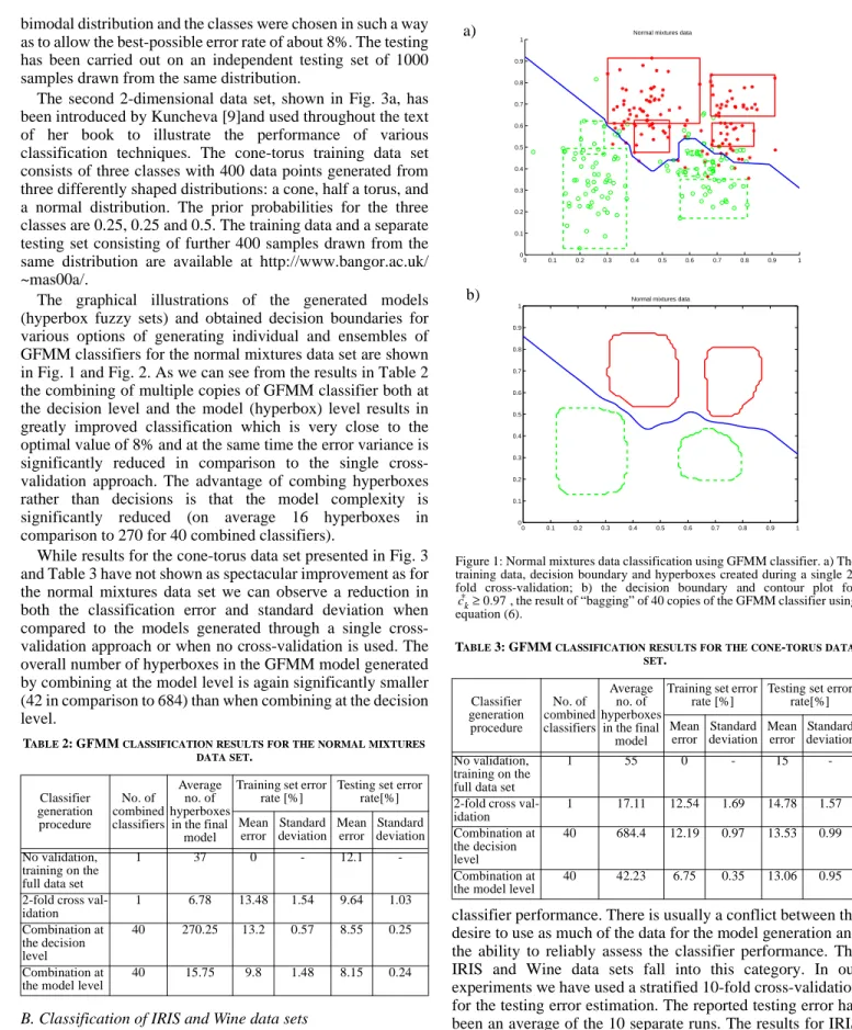
bimodal distribution and the classes were chosen in such a way as to allow the best-possible error rate of about 8%. The testing has been carried out on an independent testing set of 1000 samples drawn from the same distribution.

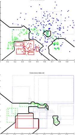
The second 2-dimensional data set, shown in Fig. 3a, has been introduced by Kuncheva [9]and used throughout the text of her book to illustrate the performance of various classification techniques. The cone-torus training data set consists of three classes with 400 data points generated from three differently shaped distributions: a cone, half a torus, and a normal distribution. The prior probabilities for the three classes are 0.25, 0.25 and 0.5. The training data and a separate testing set consisting of further 400 samples drawn from the same distribution are available at http://www.bangor.ac.uk/ ~mas00a/.

The graphical illustrations of the generated models (hyperbox fuzzy sets) and obtained decision boundaries for various options of generating individual and ensembles of GFMM classifiers for the normal mixtures data set are shown in Fig. 1 and Fig. 2. As we can see from the results in Table 2 the combining of multiple copies of GFMM classifier both at the decision level and the model (hyperbox) level results in greatly improved classification which is very close to the optimal value of 8% and at the same time the error variance is significantly reduced in comparison to the single cross-validation approach. The advantage of combing hyperboxes rather than decisions is that the model complexity is significantly reduced (on average 16 hyperboxes in comparison to 270 for 40 combined classifiers).

While results for the cone-torus data set presented in Fig. 3 and Table 3 have not shown as spectacular improvement as for the normal mixtures data set we can observe a reduction in both the classification error and standard deviation when compared to the models generated through a single cross-validation approach or when no cross-cross-validation is used. The overall number of hyperboxes in the GFMM model generated by combining at the model level is again significantly smaller (42 in comparison to 684) than when combining at the decision level.

B. Classification of IRIS and Wine data sets

While the two datasets discussed in the previous section had their dedicated separate testing sets, in most cases of real datasets there is a limited amount of data samples which have to be used both for model generation and estimation of the final

classifier performance. There is usually a conflict between the desire to use as much of the data for the model generation and the ability to reliably assess the classifier performance. The IRIS and Wine data sets fall into this category. In our experiments we have used a stratified 10-fold cross-validation for the testing error estimation. The reported testing error has been an average of the 10 separate runs. The results for IRIS and Wine data sets are shown in Table 4 and Table 5 respectively.

As we can see from the results for the IRIS data in Table 4 the performance of the classifiers generated during a 2-fold

TABLE2: GFMMCLASSIFICATION RESULTS FOR THE NORMAL MIXTURES DATA SET. Classifier generation procedure No. of combined classifiers Average no. of hyperboxes in the final model

Training set error rate [%]

Testing set error rate[%] Mean error Standard deviation Mean error Standard deviation No validation, training on the full data set

1 37 0 - 12.1

-2-fold cross val-idation 1 6.78 13.48 1.54 9.64 1.03 Combination at the decision level 40 270.25 13.2 0.57 8.55 0.25 Combination at the model level

40 15.75 9.8 1.48 8.15 0.24

TABLE3: GFMMCLASSIFICATION RESULTS FOR THE CONE-TORUS DATA SET. Classifier generation procedure No. of combined classifiers Average no. of hyperboxes in the final model

Training set error rate [%]

Testing set error rate[%] Mean error Standard deviation Mean error Standard deviation No validation, training on the full data set

1 55 0 - 15

-2-fold cross val-idation 1 17.11 12.54 1.69 14.78 1.57 Combination at the decision level 40 684.4 12.19 0.97 13.53 0.99 Combination at the model level

40 42.23 6.75 0.35 13.06 0.95 0 0.1 0.2 0.3 0.4 0.5 0.6 0.7 0.8 0.9 1 0 0.1 0.2 0.3 0.4 0.5 0.6 0.7 0.8 0.9 1

Normal mixtures data

0 0.1 0.2 0.3 0.4 0.5 0.6 0.7 0.8 0.9 1 0 0.1 0.2 0.3 0.4 0.5 0.6 0.7 0.8 0.9 1

Normal mixtures data

Figure 1: Normal mixtures data classification using GFMM classifier. a) The training data, decision boundary and hyperboxes created during a single 2-fold cross-validation; b) the decision boundary and contour plot for , the result of “bagging” of 40 copies of the GFMM classifier using equation (6).

c*_k≥0.97

a)

single cross-validation procedure is quite stable and combination either at the decision level or the model level does not improve the classification performance. It is consistent with a number of other studies of ensembles of classifiers which usually report a small increase in the classification error when ensembles are applied to this data set. The fact that the data is relatively simple and can be successfully covered by a small number of hyperboxes is illustrated in Table 4 where not only the number of hyperboxes when combining at the model level is comparable with a single 2-fold cross validation approach but it is even significantly reduced (6 in comparison to 16).

While the results for IRIS data set demonstrate that combining is not always beneficial, the results for Wine data set shown in Table 5 illustrate that the combination at the model level can also result in an increased variance. It has to be said that while the variance is increased there is also the largest improvement in the classification performance for the GFMM classifiers combined at the model level. The combination at the decision level also resulted in a significant improvement of the classification performance in comparison to models generated through a single 2-fold cross-validation procedure.

As one can also see the number of hyperboxes in different

TABLE4: GFMMCLASSIFICATION RESULTS FOR THEIRISDATA SET.

Classifier generation procedure No. of combined classifiers Average no. of hyperboxes in the final model

Training set error rate [%]

Testing set error rate[%] Mean error Standard deviation Mean error Standard deviation No validation, training on the full data set

1 22 0 - 4.67

-2-fold cross val-idation 1 16.1 2.21 0.05 3.6 0.21 Combination at the decision level 40 639.9 0.53 0.2 3.87 0.3 Combination at the model level

40 5.6 1.2 0.8 3.33 0 0 0.1 0.2 0.3 0.4 0.5 0.6 0.7 0.8 0.9 1 0 0.1 0.2 0.3 0.4 0.5 0.6 0.7 0.8 0.9 1

Normal mixtures data

0.1 0.2 0.3 0.4 0.5 0.6 0.7 0.8 0.9 1 0 0.1 0.2 0.3 0.4 0.5 0.6 0.7 0.8 0.9 1

Normal mixtures data

a)

b)

Figure 2: The results of combing 40 GFMM classifier models for the normal mixtures data. a) 262 hyperboxes after the resolving of undesired overlaps; b) the decision boundary and remaining 11 hyperboxes after retraining using 262 hyperboxes from a) as inputs to the training algorithm described in Section IIA.

TABLE5: GFMMCLASSIFICATION RESULTS FOR THEWINE DATA SET.

Classifier generation procedure No. of combined classifiers Average no. of hyperboxes in the final model

Training set error rate [%]

Testing set error rate[%] Mean error Standard deviation Mean error Standard deviation No validation, training on the full data set

1 16 0 - 9.38

-2-fold cross val-idation 1 9.82 6.11 0.34 8.28 0.65 Combination at the decision level 40 392.1 0.48 0.27 4.63 0.56 Combination at the model level

40 26 0.29 0.21 3.75 1.33 0 0.1 0.2 0.3 0.4 0.5 0.6 0.7 0.8 0.9 1 0 0.1 0.2 0.3 0.4 0.5 0.6 0.7 0.8 0.9 1

Cone torus data set

0 0.1 0.2 0.3 0.4 0.5 0.6 0.7 0.8 0.9 1 0 0.1 0.2 0.3 0.4 0.5 0.6 0.7 0.8 0.9 1

Cone torus data set

Figure 3: Cone-torus data classification using GFMM classifier. a) The training data, decision boundary and hyperboxes created during a single 2-fold cross-validation; b) the decision boundary and hyperboxes resulting from combining 40 copies of the GFMM classifier at the model level.

a)

model generation approaches follow a similar pattern for the normal-mixtures, cone-torus and Wine data sets. The number of hyperboxes when trained on a full training data set without validation is larger than for 2-fold cross validation signifying a potential overfitting of the training set. On the other hand the number of hyperboxes in the final classifier model when combining at the model level is also larger than for a single 2-fold cross-validation but the classification performance is improved. It seems that the additional hyperbox fuzzy sets in this case do not contribute to overfitting of the training data but exploit various combinations of the training samples in the areas around the class boundaries or overlapping regions. C. Acceleration of learning for large data sets by combining at the model level.

As explained in the introduction the main motivation behind combining at the model level was the high model complexity and loss of transparency of the classifier ensembles.

A slightly different example concerning an acceleration of learning for a large data set by combination at the model level is now illustrated on the basis of the SatImage data set. This data set is 36 dimensional with 6435 samples representing 6 classes. We have split the data set into 3219 training samples and 3216 testing samples. The training set has been further split into 10 stratified sets. To speed up learning only 1 out of 10 sets has been used for training while the remaining 9 are used for validation. This process has been repeated 10 times in order to use all the training data in generating classifier models. The comparative results are shown in Table 6.

As one would expect the performance of an individual GFMM classifier trained on a tenth of the training set is significantly worse than the GFMM classifier trained on the full data set. As we can see combining at the model level results in much better performance than combining at the decision level or by using individual component classifiers trained on only a tenth part of the available training set. It is clear that the 1/10th of the training data does not capture the principal properties of the data. That is why an ensemble of GFMM networks (trained on different 1/10ths of the training data) combined at the decision level performs almost as badly as a single model trained on 1/10th of the training data. On the other hand, by their nature GFMM networks (trained on different 1/10ths of the training data) combined at the model level form a single GFMM network that represents aspects of the whole data set.

This is why the GFMM networks combined at the model level in this case perform as well as a single GFMM network trained on the whole training set. What is especially interesting from our point of view is the fact that while the performance of such a classifier is comparable with a classifier trained on the full training set, the training time even on a single computer is significantly faster. It is even more interesting since it is

directly amenable for the implementation on parallel machines which should result in even further training time reductions.

V. CONCLUSIONS

An alternative approach to combination of multiple copies of the GFMM classifier has been presented. Rather than combining decisions of individual base classifiers, their models in the form of hyperbox fuzzy sets are combined. This results in a classifier with significantly reduced model complexity while preserving the improved classification performance and/or reliability observed in ensembles of classifiers. However it came at the price of increased training time since an additional training cycle had to be carried out. This involved the use of the hyperbox fuzzy sets from the models generated during a multiple cross-validation as inputs to the same learning algorithm which have been used to generate individual GFMM models. One more interesting property of combining at the model level, introduced in this paper, is the potential for accelerating the training for large data sets by using only mutually exclusive subsets of the original data set to train individual classifiers to be combined at the model level. Since the training is carried out on mutually exclusive subsets it can be easily implemented on parallel computers.

Acknowledgments

Research reported in this paper has been supported by the Nuffield Foundation grant (NAL/00259/G).

REFRENCES

[1] Breiman, L., “Bagging predictors”, Machine Learning, vol. 24, no. 2, pp. 123-140, 1996

[2] Dietterich, T.G., “Machine Learning Research: Four Current Directions”, AI Magazine, vol. 18, no. 4, pp. 97-136, 1997

[3] Dietterich, T.G., “An Experimental Comparison of Three Methods for Constructing Ensembles of Decision Trees: Bagging, Boosting, and Randomization”, Machine Learning, vol. 40, pp. 139-157, 2000 [4] Gabrys, B., “Neuro-Fuzzy Approach to Processing Inputs with Missing

Values in Pattern Recognition Problems”, submitted to Int. Journal of Approximate Reasoning (available as a Technical Report No.17, University of Paisley, Computing and Information Systems Technical Reports, ISSN 1461-6122), 2001

[5] Gabrys, B., “Data Editing for Neuro-Fuzzy Classifiers”, Proceedings of the SOCO/ISFI'2001 Conference, ISBN: 3-906454-27-4, Paisley, 2001 [6] Gabrys, B., “Agglomerative Learning Algorithms for General Fuzzy

Min-Max Neural Network”, to appear in the special issue of the Journal of VLSI Signal Processing Systems, 2002.

[7] Gabrys, B. and A.Bargiela, “Neural Networks Based Decision Support in Presence of Uncertainties”, J. of Water Resources Planning and Management, vol. 125, no. 5, pp.272-280, September/October 1999 [8] Gabrys, B. and A.Bargiela, “General Fuzzy Min-Max Neural Network for

Clustering and Classification”, IEEE Trans. on Neural Networks, vol.11, no. 3, pp. 769-783, 2000

[9] Kuncheva, L.I., Fuzzy Classifier Design, Physica-Verlag Heidelberg, 2000

[10] Ripley, B.D. Pattern Recognition and Neural Networks, Cambridge University Press, 1996

[11] Ruta, D. and B.Gabrys, “An Overview of Classifier Fusion Methods”, Computing and Information Systems (Ed. Prof. M. Crowe), University of Paisley, vol. 7, no. 1, pp. 1-10, 2000

[12] S.Theodoridis and K.Koutroumbas, Pattern Recognition, Academic Press, 1999

TABLE6: CLASSIFICATION RESULTS FORSATIMAGE DATA SET.

Classifier generation procedure No. of base_{classifiers hyperboxes}No. of _{error rate [%]}Testing set Trained on the full training set 1 566 13.24 Trained on 1/10 of the training set 1 110 20.06 Combined at the decision level 10 1105 19.02 Combined at the model level 10 345 13.49