Fast distributed first-order methods

(1)

Fast Distributed First-Order Methods

by

I-An Chen

Submitted to the Department of Electrical Engineering and Computer

Science

in partial fulfillment of the requirements for the degree of

Master of Science in Electrical Engineering

at the

MASSACHUSETTS INSTITUTE OF TECHNOLOGY

June 2012

A uthor ...

Department of Electrical Engineering and Computer Science

May 11, 2012

Certified by ...

LI/ I'

Asuman Ozdaglar

Class of 1943 Associate Professor

Thesis Supervisor

h'

Accepted by ....

Professor

Feslie

4. (olodziejski

(2)

(3)

Fast Distributed First-Order Methods

by

I-An Chen

Submitted to the Department of Electrical Engineering and Computer Science on May 11, 2012, in partial fulfillment of the

requirements for the degree of Master of Science in Electrical Engineering

Abstract

This thesis provides a systematic framework for the development and analysis of distributed optimization methods for multi-agent networks with time-varying con-nectivity. The goal is to optimize a global objective function which is the sum of local objective functions privately known to individual agents. In our methods, each agent iteratively updates its estimate of the global optimum by optimizing its local function and exchanging estimates with others in the network. We introduce dis-tributed proximal-gradient methods that enable the use of a gradient-based scheme for non-differentiable functions with a favorable structure. We present a convergence rate analysis that highlights the dependence on the step size rule. We also propose a novel fast distributed method that uses Nesterov-type acceleration techniques and multiple communication steps per iteration. Our method achieves exact convergence at the rate of O(1/t) (where t is the number of communication steps taken), which is superior than the rates of existing gradient or subgradient algorithms, and is con-firmed by simulation results.

Thesis Supervisor: Asuman Ozdaglar Title: Class of 1943 Associate Professor

(4)

(5)

Acknowledgments

This thesis owes its very existence to my advisor, Asu Ozdaglar. I am honored to be under her guidance in an area of her expertise, and I have learned a lot from her in many different ways. Her passion and dedication to research have been an inspiration to me. Our discussions have been enlightening and fruitful- especially when I'm "stuck," which happens to be more often than not, her insight gives me a fresh perspective to the problem and helps me keep a steady course. I also appreciate her kindness and encouragement even while correcting, and her patience in coaching me on critical thinking and technical writing. She has been an incredible advisor, and I would like to thank her for all the growth that resulted from working with her. I am also grateful for the support of other LIDS members. Special thanks to Ermin, for all the discussions and mentorship, both academically and personally; to Ali, Ozan, Kimon and Elie, for their helpful advice and generous encouragement, and for being such considerate officemates; to Christina, Dawsen, Henghui, Mitra, and the rest of the 6F lunch bunch, for the conversations and laughters; and to every professor, staff member and student at LIDS that I've interacted with, for making my past two years here such a wonderful experience.

Many thanks go to friends who have walked with me through these first two years of graduate school. I have been greatly blessed by brothers and sisters in the MIT Graduate Christian Fellowship and the Northwest Small Group, with whom I could share not only joys but also burdens. I am also thankful for the friendship of other Taiwanese students, and neighbors in the Sidney-Pacific residential community. Grad school may be an exciting place in itself, but it is the people encountered therein that make life here so meaningful and memorable.

Last but definitely not least, this thesis is dedicated to my parents, brothers, and the rest of my family and friends in Taiwan, who are light at the end of the tunnel for me this summer and beyond; to Jerome, for the unfailing support in word and in deed, for the unwavering patience in both good times and bad, for everything. To the only God, our Savior, through Jesus Christ our Lord, be glory, majesty, dominion,

(6)

(7)

4.1 Preliminaries . . . . 4.2 Gradient Method . . . . 4.2.1 Introduction . . . . . 4.2.2 Bound on Iterates . 4.2.3 Convergence Rate . 4.3 Proximal-Gradient Method . 4.3.1 Introduction . . . . . 4.3.2 Bounds on Iterates 4.3.3 Convergence Rate . 4.4 Beyond O(1/t) . . . . 5 Numerical Experiments 5.1 Setup . . . .

5.2 Experiments and Results . . . .

5.2.1 Step Size Choices for Single-Step Consensus . . . .

5.2.2 Convergence Rate Comparison for Single- and Multi-Step Con-sensus ... ... 6 Conclusions . . . . 5 4 . . . . 5 7 . . . . 5 7 . . . . 5 9 . . . . 6 4 . . . . 6 6 . . . . 6 6 . . . . 7 2 . . . . 7 7 . . . . 7 9 83 83 85 85 85 89

(9)

List of Figures

2-1 Comparison between subgradient and proximal-point methods . . . . 25 3-1 Error neighborhood inevitable with a constant step size: an example . 45

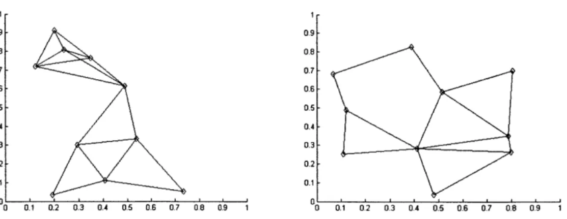
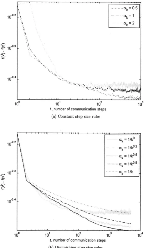
5-1 Underlying Communication Networks . . . . 85 5-2 Performance comparison under two step size rules . . . . 86

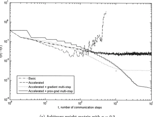
5-3 Performance comparison under two conditions for communication weight

(10)

(11)

Chapter 1

Introduction

1.1

Motivation

We live in an age with an exploding amount of information. With advances in tech-nology, we have been able to collect, store, and process data at an increasing rate and a decreasing cost. When used effectively, comprehensive information gives us a better understanding of the world and helps us improve the quality of life.

However, processing data with a single processor is often restrictive. For example, if we rely on one sensor to make measurements, it may take a long time to gather information about a vast terrain, because no matter how intricate the equipment is, it is still only able to make one measurement at a time. In such cases where information is distributed, it is much more effective to use multiple processing units, and then aggregate the message they gather.

Another limitation is in computing power. As data grow in volume, they may become computationally difficult or time-consuming to process, not to mention the additional effort required for storage and retrieval. For instance, in machine learning, a large number of training samples or features may prevent a problem from being solved effectively on a single machine. Instead, it would be desirable to leverage the power of multiple machines, each processing a portion of the data, and then combine their results.

(12)

developing distributed methods for solving optimization problems where information is decentralized among multiple agents. These methods usually involve a large number of agents connected through a network. The agents cooperatively solving a global

(convex) optimization problem through local computations and information exchange over the network. More specifically, distributed optimization methods seek to solve

min

f(x)

=

fi(x)

XERd m i=1

where m is the number of agents in the network, and for each i = 1, ..., m, fi(x) is a convex function determined by their private information. The agent i maintains xi, an estimate of the global optimum x* that minimizes the overall objective f(x).

This general form has many applications. For instance, a team of m sensors exploring an unknown environment are collaboratively solving for the parameter x, which describes the environment, by optimizing

min f(x) =

fi(x)

=

I

Ax

-

b

2

XERd TrbM J~i bl

where bi is the measurement taken at agent i and Aix is the corresponding linear transformation from the parameter space to the measurement space. Note that each agent has access to only one of the terms in the above sum.

As another example, regularized logistic regression in machine learning looks for the optimal parameter x in

min

f(x)

= E

fi(x)

= E- log(1 +exp(-by(agx)))+ 1

xERd Tr _I_NM|_N

where Ni is the training dataset of agent i, corresponding to {aj

I

j E Ni}, the set of

feature vectors, and {bj I j E Ni}, the set of associated labels.

The objective in such problems is for each agent to obtain an estimate of the global optimal solution. In reality, several constraints may prevent the agents from sharing their local function fi(x), since it encodes private information at the agent,

(13)

and may take up additional resources to transmit, process, and store. Therefore, a standard approach is to only allow agents to share their estimates xi of the optimal solution without giving away private local information contained in fi(x).

This thesis provides a systematic framework for the development and performance analysis of distributed algorithms for multi-agent optimization problems that can operate on a network with time-varying connectivity. Our development will rely on first-order methods (i.e., methods that use gradient or subgradient information), which are low-complexity alternatives to second order methods.

1.2

Related Literature

In this section, we briefly review existing algorithms and convergence rate results that are relevant to our work. Since the literature is broad, we organize our dis-cussion into three sections: centralized methods, parallel and incremental methods, and distributed methods. This is an active field with an extensive literature, and the following is not a comprehensive list, but an overview of the most relevant works.

Centralized Methods. Centralized first-order optimization methods dates back to Cauchy, who proposed the gradient method in 1847 [1]. Today, they are widely used in practice, especially in large-scale problems where higher order methods (such as Newton's method) are computationally expensive. For an objective function

F(x) : Rd -+ R that is convex and continuously differentiable, the basic gradient method generates a sequence of iterates {x}, 1 that approach x*, the optimum of

F(x), by moving the most recent iterate along the direction of steepest descent in

function value, which is opposite to the direction of the gradient. With a constant step size, it converges to the optimal solution with F(x") - F* = 0 (1/n) 1. [2]. Nesterov [3] proposed an acceleration technique that uses two previous estimates to make a prediction before performing the next gradient step. This leads to an

im-'We write g(n) = O(h(n)) if and only if there exists a positive real number M and a real number no such that |g(n)|

<5

Mjh(n)| for all n > no. Convergence rate notion are discussed in more detail

(14)

proved convergence rate of 0 (1/n 2

), which was also shown to be the best achievable convergence rate [4].

When the objective function is not differentiable, the iterates can be updated using a subgradient direction instead of the gradient direction. This is called the subgradient method. Unlike the gradient, the subgradient direction is not guaranteed to be a direction of descent, due to the fact that for nondifferentiable functions, the value of two iterates can be drastically different despite the iterates being very close. As a result, its performance is worse than that of the gradient method: with a constant step size, it converges at the best-achievable rate of 0 (1/vrn) [4].

For certain non-differentiable functions that have favorable structures allowing simple computation of the proximal operator(for example, F(x) =

I|x||1,

a common choice for regularization), the proximal-point method [51 can be applied. It utilizes desirable properties of the non-differentiable objective function to solve a minimiza-tion problem at each iteraminimiza-tion. The convergence rate of the proximal-point method is 0 (1/n 2), and it is not sensitive to step size choices. There is also the combination of both the gradient and the proximal-point method, called the proximal-gradient method, which is applicable to functions that have both a differentiable part and a non-differentiable part that have a desirable structure. It has been shown to converge

at the optimal rate of 0 (1/n 2) [6] with a constant step size.

Recently, there has also been a growing interest in stochastic approximation [7] and inexact methods [8,9]. These methods are applicable when there is error, introduced

by uncertainty or noise, in obtaining the gradient, subgradient, or in the proximal

operation. The performance of these methods can be characterized in terms of the error, and techniques for such error analysis are often useful for methods that are not centralized.

Parallel and Incremental Methods. There are several ways to divide the computation load among multiple agents. [10,11] studied the case where every agent had access to the same global objective function that is differentiable. They pro-posed a generic network communication model, analyzed its consensus properties,

(15)

and showed that a gradient-type method converged to the global optimum under this setting.

While we inherit the network communication model in [11], the parallel approach is different from our distributed setting, where the agents have private objective functions that are unknown to others.

Incremental methods, on the other hand, considers agents with private objectives who are connected via a well-structured network, and updates the iterate by passing it around the network and updating it according to each agent's private objective. [12] surveys combinations of gradient, subgradient, and proximal methods. These methods achieve exact convergence only with diminishing step sizes, and there are

currently no known techniques for acceleration in incremental gradient methods. Although they also involve agents with private objectives, incremental methods are different from distributed methods studied in this work. In incremental methods, only one agent updates at a time, whereas in distributed methods, every agent op-erates in every iteration and maintains an estimate of the global optimum, thereby utilizing full distributed computation power. Moreover, incremental methods rely on cyclic or uniformly random order of passing the iterate, while distributed meth-ods consider more generic communication networks in which agents pass iterates to multiple neighboring agents, and also combines the estimates received from different agents.

Distributed Methods. Our work is closely related to [13], which studied the distributed subgradient method with a constant step size, with convergence rate

o

(1//i). Under a similar framework, [14,15] considered constrained consensus and optimization, [16] incorporated communication link failures, [17] considered asyn-chronous updates with stochastic errors, and [18] studied the effect of graph topology on the convergence rate. Other extensions of gradient- or subgradient-based methods include [19], which considers the case where the local functions are time varying but related; and [20], which considers allows the agents to exchange gradient information rather than just estimates.

(16)

Our work extends the analysis of [13] in several ways. First, we characterize the convergence results explicitly in terms of the step size choice, giving rates for exact convergence when diminishing step sizes are used. Secondly, and more importantly, we consider proximal gradient methods instead of the subgradient method. In their centralized counterparts, as mentioned above, it has been shown that for the subgra-dient method, the convergence rate of 0 (1//n) cannot be improved, while Nesterov's techniques can applied to the proximal gradient method to accelerate the convergence rate from 0 (1/n) to 0 (1/n2). We were able to use this acceleration technique to obtain an improvement from the subgradient method.

During the preparation of of this work, [21] independently gave a distributed gradient method similar to our setting. Under a static communication network with the same weight for each neighbor, they presented a method that uses diminishing step sizes and converges exactly to the optimum at rate 0 (log n/n). In contrast, our network communication model is time-varying, and we give a method with a constant step size that converges exactly to the optimum at rate 0 (1/t) (where t is the number of communication steps taken.)

There are various other distributed methods which are extensions of other central-ized optimization methods that utilizes the dual in addition to the primal function. For example, [22] presents the dual averaging subgradient method, which allows for an explicit characterization of how the convergence rate depends on network topology. Also, [23] considers the distributed augmented Lagrangian dual method, and [24] uses an alternating direction method of multipliers (ADMM) for distributed linear regres-sion. These dual methods often involve more complicated computation, but may be more directly applicable in the context of specific problems.

1.3

Contributions

This thesis presents novel distributed methods for solving cooperative optimization problems among multiple agents connected through a potentially time-varying net-work. The goal is to optimize a global objective function which is the sum of local

(17)

objective functions, and each local objective is known by an individual agent only. We have two sets of contributions:

First, we introduce distributed proximal-gradient methods that offer flexibility in exploiting the special structure of local objective functions, enabling the use of a gradient-based scheme for non-differentiable functions with a favorable structure. We present a convergence rate analysis for such methods that highlights the dependence on the step size sequence.

We next propose a fast distributed gradient method that uses Nesterov-type ac-celeration techniques and multiple communication steps per iteration. Our method achieves exact convergence at the rate of 0(1/t) (where t is the computation time), superior than the rate achieved by existing gradient or subgradient algorithms.

1.4

Outline

The class of methods considered is outlined in Chapter 2, along with preliminary results that are important for our anaylsis.

In Chapter 3, we consider methods with a single communication step, and study the convergence properties under both constant and diminishing step sizes. For a con-stant step size rule, it extends current results for subgradient methods to proximal-gradient methods, highlighting the effect of the distributed nature of the problem on the rate of consensus. For diminishing step size rules, convergence results is charac-terized for a class of diminishing step sizes, providing an optimal choice of diminishing

step sizes within this class.

Chapter 4 offers a novel distributed gradient method that uses a constant step size, and converges with a rate of 0(1/t), where t is the number of communication steps. We explain the Nesterov-type optimization acceleration technique, as well as the effect of using multiple communication steps per iteration, both of which are crucial to achieving this result.

In Chapter 5, we present results for numerical experiments on a machine learning benchmark dataset, verifying our theoretical analysis. Chapter 6 closes with

(18)

(19)

Chapter 2

Model

This chapter sets the stage for our distributed first-order methods. In Section 2.1, we review some basics in convex analysis, including a discussion on the proximal operator. Section 2.2 describes the class of distributed methods that is the subject of our studies, followed by Sections 2.3 and 2.4 with details on its optimization and consensus aspects, respectively. In Section 2.5, we explain the convergence rate notions that will be used to characterize the performance of our methods.

2.1

Preliminaries

In this section, we gather some notations, definitions, properties and concepts that are important to our work.

Vectors and Matrices

We begin by explaining our notations and recalling some basic definitions in linear algebra.

Superscripts are used for the iteration number of vectors in our methods, for example, yk, jk , ek. Subscripts are used for the iteration number of scalars, such as

'k, k,

(20)

x E

Rd, its Euclidean norm is |xi| = (x,x), and its 1-norm is

11x11

= ZE |x(l)|,

where x(l) is its l-th entry.

For a matrix A, we denote its entry at the i-th row and j-th column as [A]Ij. We also write [aij] to represent a matrix with [A]ij = aig. A matrix is said to be stochastic

if the entries in each row sum up to 1, and it is doubly stochastic if A and A' are both stochastic.

Properties of Functions

We now list some standard definitions and properties pertaining to the class of func-tions of our interest. Details and proofs can be found in [2, Appendices A-B].

"

A function

f

: Rd

_ (-oo, oo] is convex if, for any two points

x, y E Rd, and

any t E [0, 11, we have

f (tx + (1

-

t)y) <

tf

(x) + (1

-

t)f(y).

" The effective domain of a function

f

: Rd + [-oo, oo], denoted dom(f), is defined as

dom(f)

=

{x

E

Rd I f(x) < o.

f

is said to be proper dom(f) is nonempty and the restriction of

f to dom(f)

never attains -oo. In other words,

f

: Rd + [-oo, oo] is proper if f(x) < oo for at least one x E Rd and f(x) > -oo for all x E Rd.

" A function g : Rd -+ R is continuously differentiable if its derivative exists and is continuous. It is smooth if it has derivatives of all orders. However, in the context of convex optimization, nonsmooth functions, usually refer to functions that do not even have a first-order derivative.

"

A function h

: Rd

+ (-o, cc] is lower semi-continuous if the set

(21)

is closed for every a E R.

" A function V : Rd - Rd' is called Lipschitz-continuous if there exists a constant L > 0, call the Lipschitz constant, such that

|IV(x)

- V(y)||

Lj|x

-

y||

for all x,y E Rd.

" If

f

: Rd -+ (-oo, oo] is a proper convex function, then a vector z E Rd is called

the subgradient of

f

at point x if

f(y) > f(x) + (z, y - x)

for all y E Rd. The set of all subgradients of

f

at x is called the subdifferential

and is denoted as f(x).

For a continuously differentiable real-valued convex function, the subgradient co-incides with its gradient, and we have the following characterization of convexity [2, Proposition B.3]:

Proposition 1. (Convexity of Continuously Differentiable Functions)

Let

f

: Rd -+ R be a continuously differentiable function. Then

f

is convex if and only if

f(y) > f(x) + (Vf(x), y - X)

for all x,y E Rd.

For a function with a Lipschitz-continuous gradient, we have the following well-known result [2, Proposition A.24]:

Proposition 2. (Descent Lemma)

Let

f

: Rd -+ R be a continuously differentiable function whose gradient is

Lipschitz-continuous with Lipschitz constant L(f) > 0, i.e.

(22)

for every x, y E Rd. Then for every L > L(f) and x, y E Rd,

f(x) ; f(y) + (Vf(y),x - y) +

L1x

-

yl1

2

Putting together both propositions above, we obtain the following useful expres-sion:

Proposition 3. (Convexity and Lipschitz- Continuous Gradient)

Let

f

: Rd -+ R be a continuously differentiable function whose gradient is Lipschitz-continuous with Lipschitz constant L. Then for every x, y, u E Rd,

f(u) 2 f(x) (Vf (y), u - 4) - LiX -

Y11

2

Proof. This follows directly by summing up the following expressions:

f(u) 2 f(y) + (Vf(y),u - y) (by Proposition 1)

f(y) f(x) - (Vf(y), x - y ) -

llx

-

y11

2 (by Proposition 2) 25

The Proximal Operator

The proximal operator with respect to a function

f

: Rd -+ (-oo, oo] is defined as

proxf(x) = argmin

f(z)

+

-liz

- X||2

ZERd' 2ak

In other words, the proximal operator represents the minimizer of the function

f

localized around the operand x. Note that proxy(x) = proxgf(x), so when a is not

specified, it is understood that proxf (x) = prox) (x).

(23)

the set X, with lx(x) = 0 if x E X and lx(x) = oo if x ( X. Then

x, xEX

proxyf (x) = 72x

argminzEx IIz - x| 2

,

X X

which is exactly the projection of x onto the set X. From this perspective, the proximal operator can be seen as a generalization of the projection operator. This is also why we're allowing the function

f to be an extended real-value function.

The proximal operator has the following properties:

Proposition 4. (Basic properties of the proximal operator)

Let y = prozfj(x) for some function

f

: Rd -+ (-oo, oo]. Then

(a)

(x - y) E af(y).

(b) y can be written as y = x - az, where z E

f

(y).

(c) For all u E Rd,

f(u)

f(y)

+

(X

-

yu

-

y).

Proof. (a) is clear from the observation that 0 E Of(y)

+

'(y - x) by the definition of

the proximal operator, and (b) is simply an alternative expression of (a). (c) follows

from (a) and the definition of a subgradient. 0

Another useful property of the proximal operator is that, like the projection op-erator, it is nonexpansive:

Proposition 5. (Nonexpansiveness of the proximal operator)

Let y = proxf(x) and Q = prox;(z) for some function

f

: Rd _+ (-oo, o]. Then

Py - Pro

<

||x - we|.

Proof. By Proposition 4, we have

f (D ;> f(y) + (X - y, 9 - y)

f (y) ;> fMy + (.z - y, y - y-)

(24)

whose sum is

(x-y-. + , -y) <0

which, by the Cauchy-Schwarz inequality, further implies

|| y y|2 < (X - j7 ,y ) < ||X _ - ll l|||y

-Cancelling the nonnegative term ||y - y| yields the desired result.

The proximal operator provides an alternative to the use of subgradients when optimizing nonsmooth functions. It involves finding the minimum argument z E Rd

for the expression f(z)

+

I|z

- x112, which may be difficult to calculate. However, there are certain well-structured nonsmooth functions for which this can be computed easily, and in such cases, proximal methods may outperform subgradient methods. We illustrate this by an example; more examples and applications in signal processing

can be found in [25, 2.2.2].

Consider the function

f

: R -+ R, f(x) =

Aixi,

with A > 0, and let y = prox)(x). Then, by Proposition 4, we have

{ A}, y > 0

x - y E af(y) =[-AA], y = 0

{ -A}, y < 0

We can see that the first case, x - y = A, happens only if y > 0; in other words,

y =x-A if andonlyif x-A > 0. Similarly, y =x+A if andonlyif x+A < 0. Finally, y = 0 if and only if x E [-A, A]. In summary,

(25)

which is simple to compute. It can be easily extended to the multi-dimensional one-norm

f

: Rd -+ R, f(x) = Al|x||j, which is a popular choice for regularization.

It is more effective to optimize the one-norm using the proximal operator rather than the subgradient. This is clear from comparing the following two methods for

minimizing f (x) = A x|: (Subgradient method) (Proximal-point method) x -

af(x)

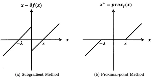
A JI 1 Z % X+ x - z, z E f(x) z+ = prox)(x) x+ X+ = pToxf (x) A __________ I

~7

-A

(a) Subgradient Method (b) Proximal-point Method

Figure 2-1: Comparison between subgradient and proximal-point methods

Figure 2-1 illustrates the update map from the previous iterate x to the next iterate

x+. When the distance from x to the minumum 0 is greater than A, both methods take a unit step towards 0. However, when x is within [-A, A], the subgradient method overshoots and in some cases may not converge to 0, while the proximal-point method brings the iterate to 0 in the following iteration and keeps it there. For this reason, the proximal operator is preferred over the subgradient when optimizing well-structured functions like the one-norm.

X

(26)

The Proximal-Gradient Method

This thesis focuses on the proximal-gradient method, which combines the use of the gradient for the continuously differentiable part of the function, and the proximal operator for the nonsmooth part. Again, these methods are particularly favorable when the proximal operator for the nonsmooth part is easy to compute.

Formally, the proximal-gradient method seeks to optimize

min f(x) = g(x) + h(x) XERd

where g : Rd -+ R is convex, continuously differentiable, and has Lipschitz-continuous gradients with Lipschitz constant L > 0, and h : Rd _ (-oo, oo] is convex, proper,

and lower-semicontinuous, but may not be differentiable.

The proximal-gradient method performs the following iterative updates:

xk = proxh{yk-1 - aV (yk-l)

It is referred to as basic if yk = xk and accelerated if yk = xk + k - xk-).

a is the constant step size, chosen such that a < . The basic method converges

with f(xk) - f(x*) = O(1/k), while the accelerated method converges with rate

O(1/k

2_{) [25].}

We highlight two properties of the proximal-gradient method that are useful for our anaylsis:

Proposition 6. (Proximal- Gradient Method) Let

X+ = pro4z{x - aVg(x)} with a < I and f (x) = g(x)

+

h(x). Then

(a) x+ can be written as

x+ = x - a (Vg(x) + z),

(27)

(b) For every u E Rd,

f (X' - f U) <1

[lix

X _U112 _

IJX+

SU 112] .

Proof. Part (a) follows directly from Proposition 4(b). As for (b), by Proposition 3,

we have

g(u) g(x+) + (Vg(x), u - x+) - 1x+ - x112

and by Proposition 4(c), we have

h(u) !h(x+ + 1(x-ag)-x+ _-X+

Summing up the two expressions above, and noting that >

,

f(u)

f(x+) +

1 X - x+,U _ X+ + _ 2

2a

Recall that for any two vectors a, b E Rd, 2 (a, b) - ||a 211 = ||b211 -

Ia

- b

1

2

.

Therefore,

f(U)

>

f(X+)+

IIIIu - X+2-

II

-x12

Rearranging terms yields the desired expression.

2.2

Distributed Proximal- Gradient Methods

Consider a network of m agents. For each i = 1, ..., m, agent i has the local objective

function

f (x) = gj(x) + hi(x)

where gi : Rd -+ R is a convex, continuously differentiable function whose gradient is Lipschitz-continuous, and hi : Rd -+ (-oo, oo] is a lower-semicontinuous proper convex function that is not necessarily differentiable.

(28)

The goal of our method is to solve the optimization problem

min

f(x)

:=

fx)

(2.1)

XERd m i=1

f(x) is called the global objective function. Its optimal value, denoted by

f*,

is assumed to be finite and attained at a unique x*.

We propose a class of first-order methods that solves the optimization problem in a distributed fashion, where each agents in the network maintains an iterate that is an estimation of the global optimum x*, using only its private objective, and the iterates of its neighbors in the network. Agent i updates its iterate as follows:

i =proxk

{wk-

1 - akVgi(w ~1)} (optimization)

2 hi I i(2.2)

Z = 1 Ajyj (consensus)

where 4, yk, 0 E Rd are vectors at agent i in iteration k, ak > 0 is the step size, and An E [0, 1] are weights.

There are two stages in this method:

" The optimization stage performs a standard proximal gradient step with the

chosen step size ak. Note that if hi(x) = 0 for each i, then the method reduces

to the gradient method.

When yk = X, it is called the basic method, and when yfC = xj+ ± (4-xi-),

it is called the accelerated method.

" In the consensus stage, each agent communicates through the network to

ex-change iterates with its neighbors. Communication may happen either only once, which we call the single-step consensus scheme, or many times, which we call multi-step consensus.

The result is modelled as a linear combination of its own iterate and that of its neighbors, and the weights A) are determined both by the communication network and by the single- or multi-step consensus scheme.

(29)

In practice, each agent only needs to maintains either y, or wi at any given time; however, for clarity of analysis, we distinguish results of the optimization and consensus stages by denoting them as y and 0f, respectively.

2.3

Conditions on Objective Functions

We assume that the functions of interest have the following properties:

Assumption 1. For every i,

(a) gi : Rd -* R is convex, continuously differentiable, and has a Lipschitz-continuous gradient with Lipschitz constant L > 0, i.e. |IVgi(x) - Vgi(y)|| <; L||x - y||.

(b) hi : R d _ (-oo, 00] is convex, proper, and lower-semicontinuous.

(c) (Bounded gradients and subgradients) There exists a scalar G such that for all x,

IVgi(x)||

< G, and ||z\| < G for each subgradient z E ah(x).

(d) (Uniqueness of optimum) f (x) = I E' 1 fi(x) = I E' 1 gi(x)

+

hi(x) attains its minimum at a unique x*.

Note that Assumption 1 implies that g(x) =

Eli

1 gi(x) and h(x) =

E

hi(x)

also satisfy the same assumptions.

While (a), (b) and (d) are standard assumptions also common to centralized first-order methods, (c) requires more justification. We now illustrate, by an exam-ple, that distributed first-order methods given in (2.2) may not converge when the

(sub)gradient is not bounded. In particular, we construct a case with unbounded gradients for the distributed gradient method, in which the estimates |x11l -+ oo as

k -± 00 for each agent i, while yk stays at the minimum of g(x) = gi. This

1M

occurs despite using a diminishing step size a. = .

We consider the most simple case with only two agents i,

j,

whose private functions are differentiable and symmetric to each other with respect of the y-axis, i.e. gi(x) =

gj (-x), hi(x) = hy (x) = 0. If we also choose a symmetric weight matrix A and

(30)

xk = - = 0 at every iteration k. We choose [Ak =1/3 2] and x - -1. Then k 1 2 k1k

1

= [3

1 [

3 for each k > 1. k 2 1 k 1. k 3_ _3 3 3 j

Next, we construct a function for which xi decreases with each step at a fixed interval. In particular, we aim at x! = -2, x? = -3, ... , x= -(k

+

1), which, by the

the previous formula, implies wk-1 =

j

We wish to have xo = 0 - g

or Vgj(j) = k(k + (k + 1)). Therefore, if we set

Vgi(x) = 3x(4x + 1) = 12x2 _{+ 3x for x > 1}

and calculate gj correspondingly, then we would end up with the desired divergent

sequence

=

-(k

+

1) -+ -oo, x -4 oo as k -4 oo. This gives V2

g, (x) = 24x + 3, so it is convex on

[-

, oo]. On the other hand, integration gives gi(x) = 4x3 + jx 2, where we have taken the integration constant to be zero for simplicity.

Finally, choose gi (x), x < 1 and gj (x), x > -1 so that they are convex and yk = 0

is the minimum of the global function gi

+

gj. We simply paste a quadratic function

of the form ax2

+ c to the left of x = I to ensure that the minimum is at 0. Using

zero- and first-order information at x = 1, Vgj(1) = 15 = 2a gj(1) - a + c 2 15 = a =- c= -2 2' Therefore, 4x3 + X2 x > 1 x2

- 2,

x

<

1

(31)

as plotted below. gj (x) = g(-x) can be constructed easily. 40-35- f(x)= 4x3 +3/2 x2,x 1 30- -- (x)= x2 - 2. x < 1 25 -20 15 10 5 0 -2 -1.5 -1 -0.5 0 0.5 1 1.5 2 X

We have thus obtained smooth convex functions for which the distributed gradient method does not converge with diminishing step sizes ak = . Indeed, without a

bound on the gradients, there are instances where the distributed method fails to converge, because there are functions whose (sub)gradients grow faster than the rate at which the step size diminishes. The most straightforward fix to this is to assume that the gradients are bounded.

2.4

Network Communication and Consensus

For the consensus stage of (2.2), we adopt the information exchange model developed in [10, 13], which we summarize in this section. In the model, the agents form a communication network, and in the communication step at time t, every agent takes a linear combination of other agents' estimates according to a weight matrix A(t) = [aij (t)]. While the weight matrix may change over time, the following conditions should always be satisfied:

Assumption 2. (Communication Network Requirements) Consider the weight matrices A(t) = [aij(t)], t = 1, 2,....

(a) (Significant weights) For every t, A(t) is doubly stochastic. Moreover, there exists a scalar 7

E

(0,1) such that for all i, agi(t) ;> 1, and for

j

= i, either agg(t) = 0,

(32)

in which case

j

is not a neighbor of i at time t, or aij(t) ;> 7, in which case

j

is a neighbor of i and receives the estimate of i at time t.

(b) (Connectivity and bounded intercommunication interval) Let

Et =

{(j,

i) |

j

_{receives the estimate of i at time t},}

Ex =

{(j,

i) |

j

receives the estimate of i for infinitely many t}.

Then E. is connected. Moreover, there exists an integer B > 1 such that if (j, i) E Eo, then (j, i) E Et U Et+₁U ... U

Et+B-1-In this assumption, part (a) ensures that each agent maintains an equal influence on and by others in the network. It also guarantees the significance of every estimate received by an agent. On the other hand, part (b) states that the overall communi-cation network is capable of passing information from an agent to any other agent in bounded time. As a result, if we take B = (m-1)B, then EtUEt+1U...UEt+--1 = Ex.

We then have the following result from [13]:

Lemma 1. [13, Proposition 1(b)] Let Assumption 2 hold, and let

4(t, s) = A(s)A(s + 1) - A(t - 1)A(t).

Then the entries [D(t, s)]ij converges to -L as t -+ oo with a geometric rate uniformly

with respect to i, j. Specifically, for all i, j E {1, ... , m} and all t, s with t > s,

m - B

For simplicity, we shall denote F = 2 1+ -, 0

<#

< 1, and quote

this theorem as

[d(t, s)]i

-

< pYk-s (2.3)

(33)

average iterate decreases geometrically with respect to the number of communication steps taken in the consensus stage. This result is crucial for our analysis later on, when showing convergence of the iterates to the average iterate.

2.5

Convergence Rate Notions

In this section, we clarify the distinction between exact convergence and convergence

to an error neighborhood, and specify two possible convergence rate notions used to

describe the latter.

Traditionally, the rate of convergence is characterized in terms of the number of iterations required to reach an E-optimal solution. x E Rd is said to be an E-optimal

solution of the function

f

: Rd -+ (-o, oo] if

f(x) -f*

For example, suppose that for a given method, the function values converge to the optimal value with a bound of

f(x") -

f* <

- (2.4)

n

for some scalar Do > 0, where n is the number of iterations. Setting the right-hand side to c, we see that it takes n = A iterations to find an e-optimal solution. In this case, we say that the method converges exactly, and the convergence rate is 0 (1/n). Another type of convergence, which usually arises in methods that use a constant step size, involves terms that depend on the step size a and do not diminish as n increases. As an example, consider the bound

f(x") -

f* <

+

D2c (2.5)

for some positive scalars D1, D2. Under the traditional E-optimality convergence rate

(34)

run, then by choosing o = to minimize

-.

+ D20, the bound becomes

V n an/DD

f(x n)f* < . n

Therefore, with a budget of n iterations, the best solution we can achieve is an NDiD2

optimal solution. In other words, to reach an c-optimal solution, at least n = VDiD2

iterations are required. In this case, since e = VDiD2, we say that the convergence

rate of this method is 0 (1/n).

While this conventional convergence rate notion provides a common basis for comparison between methods that converge exactly and methods that converge to an error neighborhood, note that it does not differentiate between the rates of (2.4) and (2.5), although they are quite different. The expression (2.4) does not require fixing a budget of iterations in advance so as to find the optimal constant step size, and it approaches the optimal solution as the method continues to run for more iterations. On the other hand, once the constant step size is fixed, (2.5) does not reach the optimal solution even if the method continues for more iterations; however, in the early stages, the rate of decrease in function value is in effect 1/n 2_{, and it may}

outperform than (2.4), until (2.4) decreases beyond the error neighborhood of (2.5). Therefore, as an alternative interpretation of convergence rate in the latter case, it is often helpful explicitly state the rate at which the error neighborhood is being reached. For example, (2.5) is also said to (2.5) converge to an error neighborhood

D2a with rate 0(1/n2). In the upcoming chapters, it should be clear from the context

(35)

Chapter 3

Distributed First-Order Methods

with Single-Step Consensus

In this chapter, we consider the distributed method where only one communication step is taken at each iteration. This is called the "single-step consensus" scheme, in-troduced in Section 3.1. In Section 3.2, we show that the basic method converges with rates O(1/Vn) for a constant step size, and O(logn/v~i) for a class of diminishing step sizes. Section 3.3 outlines challenges for using Nesterov's technique to accelerate distributed methods with single-step consensus.

3.1

Introduction

Recall from Section 2.2 that the distributed proximal-gradient method solves

min

f(x)

= E

fi(x)

= gi(x) + hi(x)

XERd m m

by iteratively performing the following:

{

4=

prox f {wz- -Vgi(-)}

wk =

r_

av k yjk

(optimization)

(consensus)

(36)

where yk = xo is call the basic method, and yi =

4f

+ k(xC - x4-1) is called the accelerated method. With single-step consensus, communication only happens once in

the consensus stage, and the weight matrices [at,] satisfy Assumption 2. The method

is initialized with {w9}T,=.

For a constant step size, [13] showed that the basic subgradient method (with

yi = x,) converges with rate O(1/vrk). We shall see that although the

proximal-gradient method makes better use of function properties in the optimization stage, it suffers from the same bottleneck due to consensus. Therefore, the convergence rate is similar to that of the subgradient method. We also extend the analysis to arbitrary step sizes and characterize the result in terms of step size choices. In particular, for the class of diminishing step sizes ak = 1/k', a > 0, we show that the best exact

convergence rate is achieved when a = 1/2.

On the other hand, in the accelerated case (with yf =

+

± (x4 - xh)), there are instances of this problem that my not converge, due to the distributed nature of this problem, and the sensitivity of the accelerated method to error. In order to take advantage of the acceleration technique, we have to control the quality of consensus

by using multiple consensus steps, which will be discussed in the next chapter.

3.2

Convergence Rate of the Basic Method

In order to derive the convergence rate of the basic proximal-gradient method, we first provide an upper bound on consensus of iterates, using properties of network communication. This is then used to derive the convergence rate, given in terms of step sizes. Finally, we characterize the rate according to the step size rule.

3.2.1

Consensus of Iterates

Recall that the goal for each agent is to maintain an estimate of the global optimum

x. If this is achieved, then the local estimates must be equal to each other, because by Assumption 1(d), x is unique. However, since each agent moves its iterate in a

(37)

the question arises as to whether local iterates will actually converge to the same point. In other words, is the single communication step in the consensus stage strong enough to "pull" the iterates close to each other?

The following lemma addresses this question:

Lemma 2. (Consensus of iterates, limited consensus) In Algorithm (3.1),

k-1

kX - yk-1 (

||w ||+

2mrG(

j=1 r=O

Yk-r-1a, +4akG

where xk = - ' x, I and -y are given in Lemma 1, and G is the bound on the

gradient of gi and the subgradients of hi for every i, as in Assumption 1.

Proof. By Proposition 6, (3.1) can be written as

X = Wk-i

[g(w-1)

_+]± (3.2)

where z E ahj(x4). Since wk-1 = a -1 x -1 due to the consensus stage, we can write (3.2) recursively: m x = a,-k kx~- [Vg(w- 1₎ +

4]

j=1 m m [k- 1, k - 2)]x-2 - a)-la._1 [Vgj(w 2_{) ±} _z-1] - ak [gi w-1) + j=1 j=1 m k-1 m = Z[4(k - 1, O)]w - j [ (k - 1, r)]ijar

[Vgj(w'-)

₊zj] - ak [Vg,(w- 1 ) + zik] j=1 r=O j=1 (3.3)

(38)

Taking the average, we have 1 yk X m _{k-1 m} ₁ 1 ₊ -wO a, [Vg_(wr-) + z

]

ak rg9 w

-

±

z1

(34

j=1 r=O j=1

where we used the fact that

Zi=

₁

[O(t,

s)]

i

= 1, since D(t, s) is doubly stochastic for

all s < t.

Subtracting (3.4) from (3.3),

I k-1 m

-x -k [D(k - 1, 0)]i[ - -O [E(k - 1,

r)]i

- jar [Vgy (wr-1) + z

]

j=1 - r-0 1

-m

- 1 k [Vg(Wh 1) ± Z ] + 1 1: Cfk [Vgj(W h) ± Zk]

Finally, taking the norm,

mm

- Xj < E11|| [4,(k - 1, 0)];g - - WO

j=1

k-1 m

+ EE [ D(k - 1, r)]i - a'Ci , gy(Wr~1)j + II0ll

r=0 j=1

+±m-l ak

(Vgi(wk-

1_)j₊_Iz _±

Zak Vg (w- 1)11 +

ZII)

i~i

7n k-1 2m-1

< rk-1 0IWII + m(k-r-12arG + 2(m-1) . 2akG

j=1 r-O m

where in the last line we used Lemma 1 and Assumption 1 (c), respectively, to bound

terms of the form

|I[D(k

- 1, r)] i - and

||Vgj(wr-

1)|| +

11zj1|.

This implies the

desired result.

The key idea behind this proof is that without the optimization stage, the algo-rithm is in effect an averaging algoalgo-rithm, and the iterates

4

= wf converge to the mean Yk. In light of this, we treat the optimization stage as a process that introduces

(39)

error to the averaging process, and study its affect on the averaging algorithm. By

(3.2), the error that occurs at each stage is

Iwk-'

- Xf|| =

jVgi(wO

1₎

+

_{z jl}_<_2akG.

From Lemma 2, it is clear that the error which happened k -r iterations ago is attenu-ated geometrically by yk-r, in line with our understanding of the consensus algorithm. This leads to the bound above.

Clearly, the choice of step sizes has a significant effect on the accumulated error. For example, if we use a constant step size, then the average error over all iterations is actually finite:

Corollary 1. (Average consensus for a constant step size)

Let ak = O in Algorithm (3.1). Then there exists scalars C1, C2 such that for

n = 1,2, ...

n n

k=1

Proof. This is obtained simply by averaging the statement of Lemma 2 over k =

1, .. n: n n m n k-1 n

E

14

-||l

<lkW

+ 2amG yk

+ E 4G

k=1 n k=1 j=1 k=1 r= k=1 < -w| + 2arG +4aG n I- 3=1

-Note that the given initial points {wojm } can be treated as known constants. Then the corollary is obtained with

F m C'1 = E

||41

j=1 1 C2' = 2amnrG + AaG 1- Y

More generally, when the step size is not constant, the error can be expressed in terms of the step sizes. The following lemma gives the total error in n iterations, in

(40)

the form that will be applied directly in the following section.

Corollary 2. (Accumulated consensus of iterates for arbitrary step sizes)

In Algorithm (3.1), there exists scalars C1,C2 such that for all iterations n =

1, 2,..,

ak Xk _ k 11 + G2 ak2 (3.5)

k=1 i=1

Proof. The accumulated consensus, weighed by step sizes ak, is

n n

)

ak k-1

+

2mPG

E

k=1 k=1 k-1 ak E r=O n 7k-r-1 r+

4G

ak 2 k=1 (3.6)

To separate the product terms, we use the fact that ab < j (a2

+

b2). Therefore,

k-1 < k=1 in <Ek 2 k=1 I 2 _n k ~+ E 72(k-1) k=1 1 ± 2 (1 - -2 7k-r-1akar n k-k=1 r=0 nk k-r-1 ₂ 2) k=1 r-O 2 n k-1 2 L ak2 k-r-1 k=1 r=0O n-1 2 2 a r=0 n k=r+1 k-r-1 n n-1 (2(1 - y) ak2+

a

1 -Y

where in the second-to-last line we swapped the order of k and r, and in the last line

we used the definition ak = 0 for k < 0 and 0k > 0 for k > 0. Substituting (3.7) and (3.8) into (3.6),

+

2mrG- 1

ak= - _k2 ₂ k=1 j=1 .k=1 n n ak 2+ 4GEak2 k=1 k=1 n ak Xk k=1 k=1

(3.7)

n Eak 2 k=1

(3.8)

(j=1 i

(41)

Gathering terms gives the statement in the corollary with C1= _{2(1 - 72)} (,=l1141 2mrG C2 = + +4G 2 1l- y 0

3.2.2

Convergence Rate Analysis

With consensus results from Corollary 2, we are now ready to evaluate the quality

of a local iterate x with respect to the global function, f(x) = -

E'i

fd()

=

1 gi(x)

+

hi(x). The result is summarized in the following theorem:

Theorem 1. (Convergence rate of the basic distributed proximal-gradient method)

Algorithm (3.1), with step sizes ak < -, maintains local estimates x with

n D1

+

D2 E k 2 fj - f* < n k=1 Zak k=1

where

fj

= min

f(x4)

is the best global

function

value obtained so

far,

f*

is the

1<k<n

optimal global function value, and D1, D2 are scalars.

Proof. Before looking at the global function f(x) =

E'i

fi(x), we first consider

the private function value of the local estimate,

fi(x)

= g;(x4)

+

hi(z4). This part

is the standard analysis inherited from the centralized proximal gradient method. Indeed, by Proposition 6 (c),

f( xu- 1 k - k-i12

ak

I

u - -2ak

=fi(z4) + 11 - U12 _ 1- _ U12]

(42)

Since the squared-norm function is convex and

w-

=E a=,-1zx- is a convex combination of {x - 1}m_1, we have

k-1 k-1_

i 1j=1

Therefore, averaging the previous expression over all i and taking u = x* to be the

global optimum, we have

fi(X )

-

fi(X*)]

2

I

x*||2

-

x

x*I 2 (3.9)

Note that the right-hand side of (3.9) is handy for recursive sums. Indeed, sum-ming (3.9) over k =

1,

.., n yields

n m M

E

[fi( ) -fi(X*)]< 1 xI- IIX *|2 L- X *|2

2

k=

mr

2 2m

k=1 = i=1

(3.10)

Returning to the global objective function, f(x) = "_1 fi(x), we wish to

eval-uate the performance of x with respect to it. However, since x is not optimized according to fi(x) for i 5

j,

the best we can do is to bound fi(x ) with

fi(x)

using convexity:

fi(xk) > f-(Xk) + (Vf,(x

),

x4

-

x)

>

fi(x )

-

G|1x1 -

xI

(3.11)

Substituting (3.11) into (3.10) bounds the global function value at xk:

n n m

ak [f(x,)

-

f*

=

(fi(x,

f(X*)]

k=1 k=1 i=1

s

: lk1][fi(x

)

+

llzIXk

_

-iX*)

k=1 i=1

< X9 - x*| + a1 ix, -- x, (3.12)

(43)

The left-hand side of (3.12) is bounded below by

\ fk) [=1 - f k= f (k)

-k=1 k=1

by the definition

f!'

= mi

f(x

).

1<k<n I

On the other hand, concerning the final term in (3.12), note that

IIX

_

X'~Il

<

llX

_ X.kII

±

lIX

_ ykII'

which leads to

mk

mi=1 I~ k1

Also, recall that by Lermma 2 we have, for all i,

ok _kIl < C1 + C2Zk 2

k=1 k=1

Therefore, utting these together,

n2 n n m Zk E

1

k=1 i=1 n -xkII

<G

aIk _ -k 11 k=1 .

<2G (C

1 +C2 L k=1

1

m I~

+

-Zakl 4 i=1 ak2

Finally, substituting (3.13) and (3.14) back to (3.12) gives the desired result:

\ Ck) [kf= --2m -, 2 i= x - x*11

+2G

C1 + C2 ak 2 \k=1 / or equivalently, Di

+

D2 Ck 2 k=1 k=1

(3.13)

G Im

--(3.14)

fjn- f*

<

(44)

where the constants are given by

2m,

Di= zZI x*2±+2GC1

D2= 2GC₂

We have thus explicitly characterized the convergence rate of the basic proximal gradient method in terms of step sizes. In the following sections, we discuss the effect of different step size rules on the convergence rate.

3.2.3

Error with Constant Step Size

Observe that if we use a constant step size, the convergence bound reduces to the following:

Corollary 3. (Convergence rate of the basic distributed proximal gradient method

with a constant step size) Consider Algorithm (3.1) with ak = a < 1. Then we have

D1/a

ffn f* _n +aD 2

where

f!, f*,

D1, D2 are defined as in Theroem 1.

The first term diminishes with the rate of O(!), similar to its centralized coun-terpart; however, instead of converging exactly to the optimum, the method is only able to converge to an error neighborhood. The size of the error neighborhood is proportional to a. Under the conventional notion of convergence rates described in Section 2.5, this amounts to a convergence rate of O(1/fri), which is the same as that of both the centralized and the distributed subgradient methods [4,13].

We next present an example showing that due to the distributed nature of the problem, an error neighborhood will be inevitable when a constant step size is used, and

Fast distributed first-order methods