Improving protein structure prediction by deep learning and computational optimization

(1)

IMPROVING PROTEIN STRUCTURE PREDICTION

BY DEEP LEARNING

AND COMPUTATIONAL OPTIMIZATION

A Dissertation presented to

the Faculty of the Graduate School at the University of Missouri-Columbia

In Partial Fulfillment

of the Requirements for the Degree Doctor of Philosophy

by JIE HOU

Professor Jianlin Cheng, Dissertation Supervisor JULY 2019

(2)

The undersigned, appointed by the Dean of the Graduate School, have examined the dissertation entitled:

IMPROVING PROTEIN STRUCTURE PREDICTION

BY DEEP LEARNING

AND COMPUTATIONAL OPTIMIZATION

presented by Jie Hou,

a candidate for the degree of Doctor of Philosophy and hereby certify that, in their opinion, it is worthy of acceptance.

Professor Jianlin Cheng

Professor Jeffrey Uhlmann

Professor Dong Xu

Professor Yunxin Zhao

(3)

DEDICATION

This dissertation is dedicated to my parents. I want to thank them for their constant support, encouragement, and love throughout my life.

(4)

ACKNOWLEDGMENTS

I would like to express my sincere appreciation to my advisor and committee chair Dr.Jianlin Cheng. Dr.Cheng constantly offered me great support and excellent suggestions during the period of my Ph.D. study. He made me passionate about my research work and encouraged me to pursue my academic goal. Without his mentoring, I could not have completed this dissertation. Dr.Cheng’s enthusiasm towards research and teaching lays the foundation for my future career.

I would like to thank my committee members for all of their guidance and sugges-tions through this long-term process, including: Dr. Dong Xu, Dr. Jeffrey Uhlmann, Dr. Yunxin Zhao and Dr. James A. Birchler.

I greatly appreciate the great support from the current and previous members in the Bioinformatics and Data Mining (BDM) lab. Their hard work and scientific contribution provided the foundation for the development of my methods. Furthermore, they created an excellent environment for research in our lab. I appreciate Dr.Jilong Li, Dr.Renzhi Cao, Dr.Badri Adhikari, and Dr.Debswapna Bhattacharya for their direct guidance in my research work. I also enjoyed working with group members including Dr.Oluwatosin Oluwadare, Meshal Alfarhood, Tianqi Wu, Chen (Chris) Chen, Anes Quadou, Adil Al-Azzawi, Zhiye Guo, and Farhan Quadir.

(5)

LIST OF TABLES

Table

Page

2.1 Performance of the six different deep architectures and their ensemble on the DNSS1 validation dataset. DNSS2 represents the ensemble of six deep architectures (CNN, RCNN, ResNet, CRMN, FractalNet and InceptionNet). . . 21 2.2 Performance of different input feature combinations on the validation

dataset of 195 proteins. PSSM, FAC, Em, Tr, HHblitsMSA denote five kinds of features: PSSM, Atchley factor, Emission probabilities, Transi-tion probabilities, amino acid probabilities from HHblits alignments. 23 2.3 Performance of the six different deep learning architectures (CNN,

RCNN, ResNet, CRMN, FractalNet, and InceptionNet) and their en-semble (DNSS2) on DNSS1 validation dataset and the updated protein sequence database. . . 23 2.4 Q3 scores of 9 secondary structure prediction methods on DNSS2 test

dataset. Three methods (SPIDER3, Porter5, DNSS2) have Q3 score higher than 85%. . . 25 2.5 Comparison of methods on the CASP13 dataset in terms of all CASP13

targets, template-based targets, and template-free targets. . . 25 2.6 Confusion matrix of helix, sheet and coil predicted by DNSS2 on CASP13

(11)

3.1 The prediction accuracy at family/superfamily/fold levels for top 1, top 5, and top 10 predictions of DeepSF and PSI-BLAST, on SCOP 1.75 test dataset . . . 44 3.2 The prediction accuracy on four validation sets with different sequence

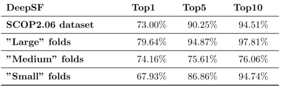
similarity to training dataset for top 1, top 5, and top 10 predictions. 45 3.3 The accuracy of DeepSF on SCOP 2.06 dataset and its subsets . . . 45 3.4 The prediction accuracy at family/superfamily/fold level for top 1, top

5, and top 10 predictions, on SCOP 2.06 test dataset. . . 46 3.5 The performance of the methods on 88 template-based proteins in the

CASP dataset . . . 47 3.6 The performance of the methods on 95 template-free proteins in the

CASP dataset . . . 47 3.7 Accuracy of protein structure predictions on 95 template-free targets. 50

4.1 The evaluation results (average ASE scores) of local quality predictions of single-model local quality QA predictors on stage 1 and stage 2 models from CASP 11. . . 70 4.2 The evaluation results (average ASE scores) of local quality predictions

of single-model local quality QA predictors on stage 1 and stage 2 models from CASP12 datasets. . . 71 4.3 The evaluation results (Corr. - Pearson’s correlation and loss) of global

quality predictions of single-model QA predictors on stage 1 and stage 2 models of CASP 11 datasets. . . 72 4.4 The evaluation results (Corr. - Pearson’s correlation and loss) of global

quality predictions of single-model QA predictors on stage 1 and stage 2 models of CASP 12 datasets. . . 73

(12)

6.1 Summary of the domain assembly performance using ab initio modeling (without SAXS) and ab initio modeling plus different SAXS-related

score functions on the 46 multidomain proteins in CASP dataset. . 137 6.2 Summary of the domain assembly performance using four domain

(13)

LIST OF FIGURES

Figure

Page

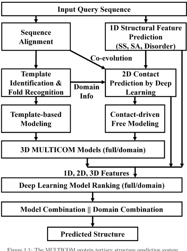
1.1 The MULTICOM protein tertiary structure prediction system . . . 4

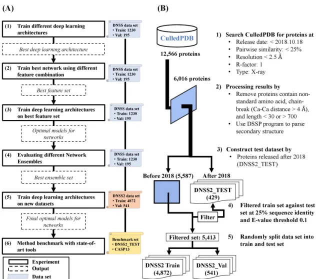
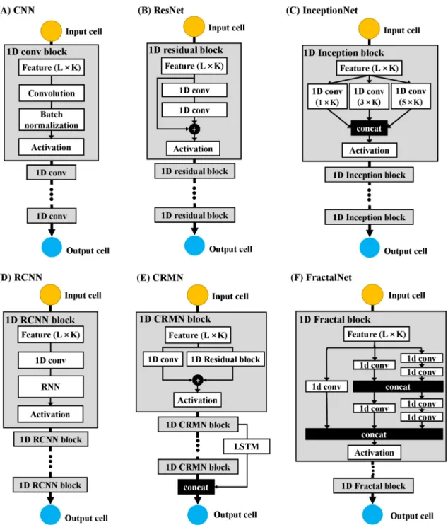
2.1 Overview of the experimental workflow for improving secondary struc-ture prediction. (A) Six principal steps are conducted to construct and train deep networks. The solid box represents an analysis step. The dashed box represents the output from the previous step. The scroll represents the dataset used in each step. (B) Dataset generation and filtering process. . . 12 2.2 Six deep learning architectures: (A) CNN, (B) ResNet, (C)

Inception-Net, (D) RCNN, (E) CRNN, (F) FractalNet for secondary structure prediction. L: sequence length; K: number of features per position. . 19 2.3 Comparison of the distribution of Q3 scores of eight existing methods

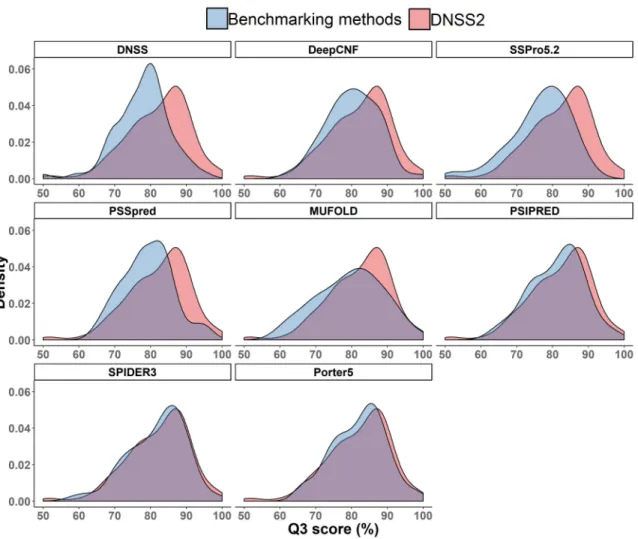
and that of DNSS2 on all CASP13 targets. . . 26

3.1 (a) The percentage of accumulated folds against length of proteins in the SCOP 1.75 dataset. In this plot, all the proteins with length less than 1,419 contains all 1,195 folds. (b) The distribution of the number of domains versus length of proteins in the SCOP 1.75 dataset. The proteins in SCOP 1.75 dataset with sequence similarity at most 95% have sequence length ranging from 9 to 1,419. . . 35

(14)

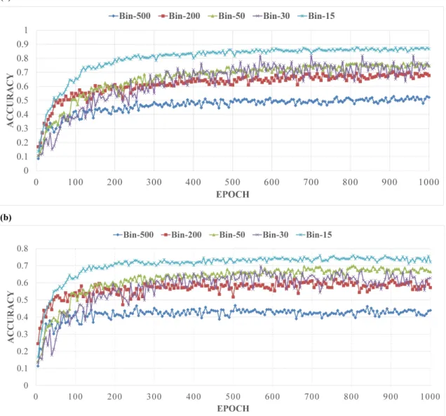
3.2 The architecture of 1D deep convolutional neural network for fold classification. The network accepts the features of proteins of variable sequence length (L) as input, which are transformed into hidden features by 10 hidden layers of convolutions. Each convolution layer applies 10 filters to the windows of previous layers to generate L hidden features. Two window sizes (6 and 10) are used. The 30 maximum values of hidden values of each filter of the 10th convolution layer are selected by max pooling, which are joined together into one vector by flattening. The hidden features in this vector are fully connected to a hidden layer of 500 nodes, which are fully connected to 1,195 output nodes to predict the probability of each of 1,195 folds. The output node uses softmax function as activation function, whereas all the nodes in the other layers use rectified linear function max(x, f(x)) as activation function. The features in the convolution layers are normalized by batches. . . 39 3.3 (a). The classification accuracy of training dataset against the number

of training epochs for 5 different bin size. (b). The classification accuracy of validation dataset against the number of training epochs for 5 different bin size. . . 43 3.4 The effects of bin size between 1 and 15 on the model training. Accuracy

was calculated based on the sequence identity reduction based dataset from SCOP 1.75. Training process was repeated and visualized as points. The averaged accuracy on the validation dataset based on each bin size was annotated. . . 44

(15)

3.5 (a) The accuracy of 4 distance metrics in clustering proteins based on fold-related features. The clustering accuracy is average over 1000 clustering processes. (b) A hierarchical clustering of proteins from 5 folds in the SCOP 2.06 dataset using KL-D as metric. Each row in the heat map visualizes a vector of fold-related hidden features of a protein. The feature vectors of the proteins of the same fold are similar and clustered into the same group. . . 49 3.6 Tertiary structure prediction for CASP12 target T0862-D1 based on

templates identified by DeepSF and HHSearch. (a) DeepSF predictions: a top template, five predicted folds and the supposition between the best model and the template structure; (b) HHSearch predictions: top template, and superposition of the best model and the template structure. . . 51 3.7 The KL-D divergences of fold-related features of 106 modified sequences

of protein ’d1lk3h2’ from the wild-type sequence (red dots) and those of 500 random sequences from the wild-type sequence (blue dots). . 53 3.8 (a). The KL-D divergences of fold-related features of 102 modified

sequences of protein ’d1foka3’ from the wild-type sequence (red dots) and those of 500 random sequences from the wild-type sequence (blue dots). We generated 46 sequences with at least one residue deleted, and 40 sequences with at least one residue insertion, and 16 sequences with at least one residue mutation. (b). The KL-D divergences of fold-related features of 106 modified sequences of protein ’d1ipaa2’ from the wild-type sequence (red dots) and those of 500 random sequences from the wild-type sequence (blue dots). We generated 45 sequences with at least one residue deleted, and 41 sequences with at least one residue insertion, and 20 sequences with at least one residue mutation. 54

(16)

3.9 The feature importance analysis on fold classification. Accuracy was calculated based on the sequence identity reduction based dataset from SCOP 1.75. Training process was repeated and visualized as points. The averaged accuracy on the validation dataset based on each feature set was annotated. . . 56

4.1 The architecture of 1D deep convolutional neural network for protein model quality prediction. (A). The network (LocalQA-net) accepts the raw features of models of proteins of variable sequence length (L) as input, and transforms the features into higher-level hidden features by 5 hidden layers of convolutions. Each convolutional layer applies 5 filters to windows of previous layers to generate L hidden features. The window size for each filter is set to 6. The last output layer adds one convolutional layer with one filter to generate the output of length L representing the local quality for each of L residues. . . 66

(17)

4.2 The architecture of 1D deep convolutional neural network for protein model quality prediction. (B). The network (InteractQA-net) contains a common sub-network for extracting features from the input layer by convolution and two sub-networks for local quality (LocalQA-net) and global quality (GlobalQA-net) predictions separately. The network accepts the raw features of models of proteins of variable sequence length (L) as input, and transforms the features into higher-level hidden features by 10 hidden layers of convolutions. Each convolutional layer applies 10 filters to windows of previous layers to generate L hidden features. The window size for each filter is set to 15. LocalQA-net adds one convolutional layer with one filter at the top of the common sub-network to generate the output of length L representing the local quality for each of L residues. GlobalQA-net uses one 30-max pooling layer to select 30 maximum values from the output of each filer in the last layer of the common sub-network as features, which are joined together into one vector by a flatten layer. The flatten layer is fully connected to a hidden layer whose output is used by a single output node to predict the global quality score. LocalQA-net and GlobalQA-net are trained by local quality scores and global quality scores alternately. . . 67 4.3 The architecture of 1D deep convolutional neural network for protein

model quality prediction. (C). JointQA-net accepts the features of protein models of variable sequence length (L) as input and predicts the L local quality scores and one global quality score simultaneously. The weights in the network are optimized by both local and global quality scores at the same time. . . 68

(18)

4.4 The comparison of local quality predictions of the method trained in different situations: (1) with Rosetta energy, (2) without Rosetta energy, (3) using only single-domain models in training, and (4) using both single-domain and multi-domain models (all models of all targets) in training. . . 75 4.5 Residue-specific distance error predicted by our method (Green) and

the real distance error between predicted model and native structure (Gray). (A) The distance error at each amino acid position in the predicted local quality and in the predicted model of T0843. (B) The superimposition of the predicted structure (Green) of the model for target T0843 and its native structure (Gray). The red highlighted regions are the major deviation between predicted model and native structure, matching the large predicted deviation in the local quality prediction. (C) The distance error at each amino acid position in the predicted local quality and in the predicted model of T0861. (D) The superimposition of the predicted structure (Green) of the model for target T0861 and its native structure (Gray). . . 77

5.1 The pipeline of MULTICOM server and human prediction systems. 86 5.2 The pipeline of DNCON2 for protein residue-residue contact distance

prediction. The input volume has 56 channels (matrices) containing various pairwise residue-residue features. . . 87 5.3 Automated contact distance-based ab initio protein structure prediction

by CONFOLD2. . . 90 5.4 The workflow of deep learning-based model quality assessment with

(19)

5.5 Evaluation of four MULTICOM predictors. The methods are ranked by average TM-score of the first (i.e., TS1) submitted models. (A) on 104 domains (Left plot: TM scores of MULTICOM, MULTICOM CLUSTER, MULTICOM-NOVEL models versus TM scores of MULTICOM-CONSTRUCT models; Right plot: mean and variation of the TM-scores of the models

of the four methods). (B) on 40 template-based (TBM-easy) domains. (C) on 31 template-free (FM) domains. . . 95 5.6 Comparison of DeepRank with individual QA methods used in

MUL-TICOM predictors. (A) The box plot of loss of each method. Here the loss is measure at 1-point scale (i.e., the highest/perfect GDT-TS score = 1). (B) The GDT-TS score at the 100-point scale of the top models selected by each individual QA method and DeepRank is plotted against the GDT-TS score of MULTICOM’s first submitted models for 74 ”all group” full-length targets. The curve for each method is fitted by the second-degree polynomial regression function. The area under the curve for each method is calculated and shown on the top left. The larger area indicates the better capacity of model selection. . . 98 5.7 Tertiary structure prediction for T0966. (A) The distribution of

GDT-TS scores of 146 server models. (B) The plot of the true GDT-GDT-TS scores of models against their predicted ranking by MULTICOM. The point highlighted in red is the top model selected by DeepRank. (C) The native structure of target T0966 (PDB code: 5w6l). (D) The top selected model. (E) The final first MULTICOM model (TS1). . . . 99

(20)

5.8 The modeling performance of contact-based ab initio modeling methods versus the predicted contact accuracy (L/5 contacts) in CASP13. Each point represents the modeling accuracy in terms of GDT-TS score versus the accuracy of predicted contacts for a method. The colors represent different modeling methods. Rosetta without contacts (purple) was included for comparison. The averaged GDT-TS score and TM-score of five methods on the all CASP13 targets are summarized in the top-right table. . . 101 5.9 A successful ab initio modeling example (a domain of target T1000) for

which no significant templates were identified. For the FM domain of T1000 (residues 282-523), the accuracy of top L/5 predicted contacts is 100%, top L 79% and top 2L 50%. CONFOLD2 successfully built a complicated α-helix+β-sheet+α-helix model for the domain with TM-score of 0.8 and GDT-TS of 0.64, while RosettaCon failed to generate a correct topology (i.e., TM-score = 0.33 <0.5 threshold). This example shows that the pure contact distance driven method such as CONFOLD2 can build high-quality structural models of complicated topology for large domains if a sufficient number of accurate contact predictions are provided. . . 102 5.10 The successful modeling of a large multi-domain target T0996 and the

contact-based validation. The contacts (red) predicted by DNCON2 match with the contacts (blue) in the template-based models domain by domain. . . 105 5.11 The input web page of MULTICOM web server. . . 109 5.12 The MULTICOM web server’s prediction for CASP13 target ”T0951”.

(21)

5.13 The native structure (shown in green color) and MULTICOM-predicted structure (shown in blue color) superimposed using Chimera for target T0951 (PDB code: 5z82) . . . 114 5.14 The MULTICOM web server’s prediction for CASP13 target T1022s1.

The orange boxes annotate different prediction results. The target was predicted to have two domains. . . 117 5.15 The MULTICOM web server’s prediction for the first domain of T1022s1. 118 5.16 The MULTICOM web server’s prediction for the second domain of

T1022s1. . . 119

6.1 Parameterization of conformation in linker regions and overall shape match with SAXS data. . . 131 6.2 Average Pearson correlation coefficient between the structural quality

(RMSD) and the SAXS score functions derived from (a) full-atom and (b) Cα atom models of protein structure. Analysis was done based on

the predicted models from CASP8-11. . . 133 6.3 Comparison of five SAXSDom approaches with the SAXSDom-abinitio

method (does not use SAXS) on the best 50 assembled models. (A) SAXSDom (Esaxs) versus SAXSDom-abinitio (Left plot: TM scores of SAXSDom (Esaxs), models versus TM scores of SAXSDom-abinitio models; Middle plot: RMSD of the models of the two methods; Right plot: Distribution ofχ score of all assembled models for 46 proteins by two methods (mark the 2 curves in the plot). (B) SAXSDom (Esaxs·χ) versus SAXSDom-abinitio. (C) SAXSDom (Esaxs·P r) versus SAXSDom-abinitio. (D) SAXSDom (Esaxs·Rg) versus SAXSDom-abinitio. (E) SAXSDom (Esaxs·IntF it) versus SAXSDom-abinitio. . . 136

(22)

6.4 Comparison of SAXSDom with SAXSDom-abinitio, AIDA and Modeller on the best of 50 assembled models. (A) SAXSDom versus SAXSDom-abinitio (Left plot: TM scores of SAXSDom models versus TM scores of SAXSDom-abinitio models; Middle plot: RMSD of the models of the two methods; Right plot: Distribution of χscores of all assembled models for 46 proteins by two methods). (B) SAXSDom versus AIDA. (C) SAXSDom versus Modeller. . . 139 6.5 The predicted assembly models and shape envelops of five two-domain

proteins. The predicted model (colored) and the native structure (green) is superimposed. The domain linker (yellow) and domains (purple, red) are highlighted in the predicted model. (A) The signal recogni-tion particle receptor from E. coli (chain A of 1FTS), linker length = 9, RMSD=2.8, TMscore=0.88, χ score=2.8. (B) The rRNA methyl-transferase ErmC’ (chain A of 1QAM), linker length = 4, RMSD=2.9, TMscore=0.81, χ score=1.6. (C) Protein of unknown function from Bacteroides ovatus (chain A of 3P02), linker length = 4, RMSD=3.4, TMscore=0.81, χ score=1.7. (D) Myo-inositol monophosphatase (chain A of 2BJI), linker length = 7, RMSD=2.7, TMscore=0.86,χscore=0.70. 141 6.6 Comparison of predicted models for 1FTS by SAXSDom,

SAXSDom-abinitio, AIDA and Modeller. (A) The SAXS profiles calculated from the models and the experimental structure. (B) The assembled full-length model with quality measurements. (C) Residue-by-residue distance error between the predicted models and the experimental structure. 142

(23)

ABSTRACT

Protein structure prediction is one of the most important scientific problems in the field of bioinformatics and computational biology. The availability of protein three-dimensional (3D) structure is crucial for studying biological and cellular functions of proteins. The importance of four major sub-problems in protein structure prediction have been clearly recognized. Those include, first, protein secondary structure predic-tion, second, protein fold recognipredic-tion, third, protein quality assessment, and fourth, multi-domain assembly. In recent years, deep learning techniques have proved to be a highly effective machine learning method, which has brought revolutionary advances in computer vision, speech recognition and bioinformatics.

In this dissertation, five contributions are described. First, DNSS2, a method for protein secondary structure prediction using one-dimensional deep convolution network. Second, DeepSF, a method of applying deep convolutional network to classify protein sequence into one of thousands known folds. Third, CNNQA & DeepRank, two deep neural network approaches to systematically evaluate the quality of predicted protein structures and select the most accurate model as the final protein structure prediction. Fourth, MULTICOM, a protein structure prediction system empowered by deep learning and protein contact prediction. Finally, SAXSDOM, a data-assisted method for protein domain assembly using small-angle X-ray scattering data. All the methods are available as software tools or web servers which are freely available to the scientific community.

(24)

Chapter 1

Introduction

Three-dimensional (3D) structure information of proteins is vital for studying their function involved in the cellular processes. The uniquely folded three-dimensional (3D) conformation (tertiary structure) of a protein is primarily determined by its amino acid sequence. Over the past decade, the advancement of high-throughput DNA sequencing technology has drastically reduced the cost and time of genome sequencing and produced tens of millions of protein sequences [1]. However, determining 3D protein structure through experimental techniques (i.e., X-ray crystallography, or NMR spectroscopy) is still time-consuming, labor-intensive and rather expensive, leaving most proteins without solved structures. The gap between the number of protein sequences and experimentally determined structures is exponentially enlarged [2]. Therefore, developing effective and accurate computational tools that can predict protein structure from its amino acid sequence is one of the most important tasks in bioinformatics and computational biology.

Computational methods for protein structure prediction can be classified as template-based and template-free (ab initio). Template-based modeling methods (TBM) attempt to build the tertiary structure of a target protein by using the known

(25)

modeling or comparative modeling. These methods are able to generate accurate three-dimensional structures if the homologous proteins with known structures can be accurately detected and well aligned with a target protein. Otherwise, it cannot predict the correct structure. Ab initio protein structure prediction is to predict the 3D structure from protein sequence without using known structures as template. Fragment-assembly based modeling is one of the representative ab initio methods for structure prediction [6]. Even though it can predict correct structures for some small proteins, it often fails to build the structures of medium to large proteins with complicated topology. Ab initio protein structure prediction has achieved major breakthroughs in the recent years due to the drastic improvement of the accuracy of residue-residue contact distance prediction based on the co-evolutionary analysis and deep learning [7, 8, 9, 10]. The distance-geometry based ab initio modeling using predicted contact distances as restraints is able to build correct structures of proteins of large size and with complicated topologies on various benchmarks and the recent Critical Assessments of Techniques for Protein Structure Prediction (CASP) [4, 10, 11]. In addition to model construction by template-based modeling or ab initio modeling, model quality assessment and model refinement are also two integral parts of a protein structure prediction system [12, 13, 14].

Figure 1.1 is an overview of our protein structure prediction system [4]. Given a target protein sequence, our method first generates the multiple sequence alignments (MSA) by searching the sequence against the non-redundant sequence database to build sequence profiles (i.e. position specific scoring matrix (PSSM) and hidden Markov model (HMM)) for protein templates identification [15] and multiple sequence align-ments for co-evolutionary analysis and two-dimensional(2D) residue-residue contact predictions at multiple distance thresholds (i.e. 6 ˚A, 7.5 ˚A, 8 ˚A, 8.5 ˚A, and 10 ˚A) [8]. The sequence profiles are also used to predict several important one-dimensional(1D) protein features including secondary structure, solvent accessibility and disorder

(26)

re-gions [16, 17]. The profile or sequence of the target was searched against the template profile/sequence library by a number of sequence alignment tools and classifying protein sequences into folds using deep learning to identify protein templates whose structures were known. The sequence alignments between the target and the identified templates are also used to predict domain boundaries. The regions of the target not aligned with any significant template are modeled by template-free (ab initio) methods with contacts (i.e. CONFOLD2, ROSETTA, UniCON3D and FUSION) [6, 10, 18, 19], and the regions covered by templates are modeled by the multi-template combination modeling approach [3, 20]. Both the fragment-assembly and distance-geometry based ab initio modeling methods are used with predicted contacts to make 3D structure prediction when the target sequence does not have significant templates. A number of structures (i.e. generally more than 100 structures) are generated from various target-template alignments produced by a variety of sequence alignment algorithms or their combinations [21]. Model evaluation plays an important role in protein structure prediction, which evaluates the quality of a protein model without knowing its true structure. We use a deep-learning-based quality assessment method to select the presumably most accurate structural models from all these predicted models. The structure of the selected model is then refined using the model refinement techniques [14].

In this dissertation, I mainly focus on my research of applying deep learning and computational optimization methods for protein structure modeling and model quality assessment, which are two principal problems in bioinformatics. Five contributions are described−(a) DNSS2, a method for protein secondary structure prediction using one-dimensional deep convolution network, (b) DeepSF, a method of applying deep convolutional network to classify protein sequence into one of thousands known folds, (c) CNNQA & DeepRank, two deep neural network approaches to systematically evaluate the quality of predicted protein structures and select the most accurate

(27)

(28)

model as the final protein structure prediction, (d) MULTICOM, a protein structure prediction system empowered by deep learning and protein contact prediction, (e) SAXSDOM, a data-assisted method for protein domain assembly using small-angle X-ray scattering data.

Chapter 2 of this dissertation mainly describes the deep learning application in protein secondary structure prediction. We designed several advanced one-dimensional deep convolution networks to predict secondary structures (e.g., deep convolutional/ recurrent/residual/memory/fractal/inception networks). The main content is from the following deposited paper:

Hou, J., Guo, Z., & Cheng, J. (2019). DNSS2: improved ab initio protein secondary structure prediction using advanced deep learning architectures. bioRxiv, 639021. [22]

Chapter 3 will describe the deep learning application for protein fold recognition. We developed a new deep-learning-based methods to improve template identification for hard proteins that have little sequence similarity with known structures. Instead of using traditional approaches that identify protein pairs with the same fold based on their pairwise sequence/profile similarities, we utilized the learning power of deep learning to directly classify the target protein to one of thousands of folds. This improved the sensitivity of detecting remote homologous proteins that share the same fold. This chapter is mainly from the content of published paper as follows:

Hou, J., Adhikari, B., & Cheng, J. (2017). DeepSF: deep convolutional neural network for mapping protein sequences to folds. Bioinformatics, 34(8), 1295-1303.[23]

Chapter 4 describes a novel single-model quality assessment (QA) method CNNQA, which predicts the absolute local quality of a single protein model based on a deep one-dimensional convolutional neural network (1DCNN). The main content of this

(29)

chapter is from the following deposited paper:

Hou, J., Cao, R., & Cheng, J. (2019). Deep convolutional neural networks for predicting the quality of single protein structural models. bioRxiv, 590620.[24]

Chapter 5 describes a new deep-learning-based consensus method (DeepRank) for protein quality assessment that integrates multiple QA methods and residue−residue contact predictions for predicting the global quality of models. The method shows a significant improvement compared to the individual QA methods used to generate input features and is more consistent in selecting models of better quality. This method was officially ranked No.1 in ranking protein structural models in the 13th Critical Assessment of Techniques for Protein Structure Prediction (CASP13).

In chapter 5, we also describe the method of our protein structure prediction system (MULTICOM) which is driven by deep learning and contact prediction. The method was officially ranked 3rd _{out of all 98 human and server predictors in CASP13} (2018). The main content of this chapter comes from the following publication:

Hou, J., Wu, T., Cao, R., & Cheng, J. (2019). Protein tertiary structure modeling driven by deep learning and contact distance prediction in CASP13. Proteins: Structure, Function, and Bioinformatics. [4]

Chapter 6 describes a novel framework of applying machine learning and com-putational optimization approaches to improve the protein domain assembly by incorporating experimental restraints from small-angle X-ray scattering (SAXS) data. The main content is from the following deposited paper:

Hou, J., Adhikari, B., Tanner, J. J., & Cheng, J. (2019). SAXSDom: Modeling multi-domain protein structures using small-angle X-ray scattering data. bioRxiv, 559617. [25]

(30)

Chapter 2

DNSS2: improved ab initio protein

secondary structure prediction

using advanced deep learning

architectures

2.1

Abstract

Accurate prediction of protein secondary structure (alpha-helix, beta-strand and coil) is a crucial step for protein inter-residue contact prediction and ab initio tertiary structure prediction. In a previous study, we developed a deep belief network-based protein sec-ondary structure method (DNSS1) and successfully advanced the prediction accuracy beyond 80%. In this work, we developed multiple advanced deep learning architectures (DNSS2) to further improve secondary structure prediction. The major

improve-ments over the DNSS1 method include (i) designing and integrating six advanced one-dimensional deep convolutional/recurrent/residual/memory/fractal/inception net-works to predict secondary structure, and (ii) using more sensitive profile features inferred from Hidden Markov model (HMM) and multiple sequence alignment (MSA).

(31)

Most of the deep learning architectures are novel for protein secondary structure prediction. DNSS2 was systematically benchmarked on two independent test datasets with eight state-of-art tools and consistently ranked as one of the best methods. Particularly, DNSS2 was tested on the 82 protein targets of 2018 CASP13 experiment and achieved the best Q3 score of 83.74% and SOV score of 72.46%. DNSS2 is freely available at: https://github.com/multicom-toolbox/DNSS2.

2.2

Introduction

Three major types of protein secondary structure are alpha-helix (H), beta-strand (E) and coil state (C) [26], each of which represents the local structure state of an amino acid in a folded polypeptide chain. The predicted information of protein secondary structure is useful for many applications in computational biology, such as protein residue-residue contact prediction [8, 9, 27], protein folding [23, 28, 29], ab-initio protein structure modeling [6, 10, 30] and protein model quality assessment [31, 32]. For instance, secondary structure prediction was widely utilized in the template-based structure modeling through threading or comparative modeling on those proteins that have structurally determined homologs [3, 5, 30], and in ab-initio modeling for those proteins whose sequences share few sequential similarities with known solved structures [33, 34].

The progress in protein secondary structure prediction over the past few decades can be generally summarized from two aspects: the discovery of novel features that are useful for prediction and the development of effective machine learning algorithms [35, 36]. The early attempts utilized statistical propensities of single amino acid observed from known structures to identify secondary structures in proteins [37]. The subsequent improvements came from the inclusion of sequence evolutionary profile features inferred from multiple sequence alignment (MSA) such as position-specific

(32)

scoring matrices (PSSM) [16, 38, 39, 40, 41, 42]. In addition to the PSSM, the Hidden Markov model (HMM) profiles derived from HHblits [15] was proposed for predicting protein structural properties [43]. Atchley’s factors were also included in some studies to capture the similarity between the types of amino acids [44, 45].

Meanwhile, the machine learning algorithms for protein secondary structure pre-diction also continued to improve. Several early approaches applied shallow neural networks [46, 47], information theory and Bayesian analysis [48, 49, 50] to secondary structure prediction. PSIPRED [40] method proposed a two-stage neural network to predict the secondary structure from the PSI-BLAST sequence profiles. SSpro [42] used bi-directional recurrent neural networks to capture the long-range interactions between amino acids. Deep learning techniques recently achieved significant success in secondary structure prediction [39, 51, 52, 53, 45, 54]. DNSS [45] applied an ensemble of deep belief networks to predict 3-state secondary structure. SPIDER2 [55] em-ployed stacked sparse auto-encoder neural networks to predict the several structural properties iteratively, and this method was further advanced by bidirectional long- and short-term memory (LSTM) neural networks to capture the long-range interactions [53]. DeepCNF [54] integrated the convolutional neural networks with conditional random-field to learn the complex sequence-structure relationship and interdepen-dence between sequence and secondary structure. Porter 5.0 [56] ensembled seven bidirectional recurrent neural networks to improve the protein structure prediction. Assisted with the power of deep learning, the accuracy of 3-state secondary structure prediction has been successfully improved above 84% [51, 53, 54] on some benchmark datasets.

In this work, we developed an improved version of our ab initio secondary structure method using multiple advanced deep learning architectures (DNSS2). Three major improvements have been made over the original DNSS method. Firstly, besides the PSSM profile features and Atchley’s factors used in DNSS, we incorporated several

(33)

novel features such as the emission and transition probabilities derived from Hidden Markov model (HMM) profile [15], and profile probabilities inferred from multiple sequence alignment (MSA) [16]. All the three new features represent the evolutionary conservation information for amino acids in sequence. Secondly, we designed and integrated six types of advanced one-dimensional deep networks for protein secondary structure prediction, including traditional convolutional neural network (CNN) [57], recurrent convolutional neural network (RCNN) [58], residual neural network (ResNet) [59], convolutional residual memory networks (CRMN) [60], fractal networks [61], and Inception network [62]. The ensemble of six networks from DNSS2 significantly improved the secondary structure prediction. Finally, DNSS2 was trained on a large dataset, including 4,872 non-redundant protein structures with less than 25% pairwise sequence identity and 2.5 ˚A resolution. Our method was extensively tested on the independent dataset and the latest CASP13 dataset with other state-of-art methods and delivered the state-of-the-art performance.

2.3

Materials and Methods

2.3.1

Experimental design

In this work, the main objective was to improve the secondary structure prediction by developing more advanced deep learning architectures and introducing more useful features. In the process, we have developed a systematic framework to effectively build deep learning architectures and obtain features to improve secondary structure prediction. Figure 2.1 provides an overview of our experimental design. Figure 2.1(A) lists the six major steps of designing, training and testing deep learning architectures. Figure 2.1(B)illustrates the process of creating training and validation datasets. The key analysis is to design appropriate architectures and investigate if they

(34)

can improve prediction accuracy. Six different deep neural network architectures were evaluated in the study, including convolutional neural network (CNN) [57], recurrent convolutional neural network (RCNN) [58], ResNet [59], convolutional recurrent memory network (CRMN) [60], FractalNet [61], and Inception network [62]. Most of these architectures were applied to secondary structure prediction for the first time. The detailed description of each network is included in Section 2.3.4. To ensure a fair comparison, each network was optimized using the original feature profiles of training proteins and evaluated on the same validation set of DNSS1. The network that achieved the best Q3 accuracy was selected to explore the feature space on the profiles derived from multiple sequence alignments (MSA) generated by PSI-BLAST [38] and HHblits [15], Atchley factors, and emission/transition probabilities inferred from the Hidden Markov model (HMM) profile. The optimal feature set was determined according to the highest Q3 accuracy on the validation datasets. The networks were then re-trained using the optimal input profiles to obtain the best models.

Since combining predictors generally improved the prediction accuracy, the different combinations of networks were also evaluated. Finally, after the optimal sets of deep learning architectures and feature profiles were determined, all networks were re-trained on the large dataset that was manually curated including the non-redundant proteins whose structures have been released publicly before 2018. The final networks were used to predict the secondary structure for the test proteins. The probabilities of the three states (i.e., helix, sheet, and coil) for each residue predicted by six networks were averaged to make the final secondary structure prediction. Our method was then benchmarked with other state-of-art methods on the two independent test datasets.

2.3.2

Datasets and evaluation metric

(35)

Figure 2.1: Overview of the experimental workflow for improving secondary structure prediction. (A) Six principal steps are conducted to construct and train deep networks. The solid box represents an analysis step. The dashed box represents the output from the previous step. The scroll represents the dataset used in each step. (B) Dataset generation and filtering process.

(36)

and 195 validation proteins was utilized to investigate whether the deep learning architectures and novel features can boost the prediction accuracy.

To utilize more data available since DNSS1 was published, a new, larger training set of DNSS2 was constructed from CullPDB [63] curated on 18 October 2018 (Figure 2.1(B)). The dataset consists of 12,566 proteins that share less than 25% sequence identity with 2.5 ˚A resolution cutoff and R-factor cutoff 1. The structures of all the proteins were determined by X-ray crystallography. The dataset was then filtered by removing proteins with non-standard amino acids, chain-break (i.e., distance of adjacent Ca-Ca atoms is larger than 4 ˚A), and sequence length shorter than 30 or longer than 700 amino acids. Considering all external methods benchmarked in this work were developed prior to year 2018, the proteins that were released after Jan 1st, 2018 were extracted as independent test set (DNSS2 TEST). The resulting set of proteins was further filtered against DNSS2 TEST set using CD-HIT suite [64] with criteria of 25% sequence identity cutoff and e-value threshold 0.1. Finally, 5,413 proteins released prior to Jan 1st, 2018 were obtained as our training set, in which 4,872 proteins were used for network training (DNSS2 TRAIN) and 547 proteins were used for model selection (DNSS2 VAL). In addition, the proteins of the CASP13 (2018) experiment were collected and the ones with at least 25% sequence identity with training proteins were removed, which results in a set of 82 test proteins. The proteins were also classified into template-based (TBM) and free-modeling (FM) targets based on the official CASP definition (CASP 13, 2018, http://www.predictioncenter.org/casp13/index.cgi). In summary, the final test set contain 429 proteins from DNSS2 TEST and 82 proteins from CASP13.

We evaluated our secondary structure prediction based on two primary metrics: Q3 accuracy and Segment Overlap measure (SOV). Q3 score represents the percent of correctly predicted secondary structure states in a protein. SOV score measures the similarity between the predicted segments of continuous structure states and those

(37)

in the experimental structure [45, 65]. The Q3 and SOV scores are complementary with each other for secondary structure evaluation. All training and testing proteins’ structure files were parsed by DSSP program [66] to obtain the real secondary structure classification for each amino acid for training and evaluation.

2.3.3

Input features

The profile of each amino acid is represented by 21 numbers from PSI-BLAST-based position specific scoring matrix (PSSM), 20 emission probabilities and 7 transition probabilities extracted from Hidden Markov Model (HMM) profile, 20 probabilities of standard amino acid calculated from the multiple sequence alignment (MSA) and 5 numbers derived from Atchley’s factor. These features (73 numbers in total) represent the evolutionary conservation and physicochemical properties for residues in a protein sequence.

PSI-BLAST was run to generate multiple sequence alignment and PSSM profile through searching a sequence against filtered UniProt sequence database at 90% sequence identity (UniRef90) [67] with three iterations and an e-value cutoff 0.001 (’-evalue .001 -inclusion ethresh .002’). Less stringent threshold was used (’-evalue 10 -inclusion ethresh 10’) in case some proteins did not have homologous sequences returned. In a PSSM profile, each position is represented by 20 numbers related to the probabilities for 20 standard amino acids appearing at the position in the multiple sequence alignment. In addition, the sequence information in the second to the last column in PSI-BLAST profile is given for each residue. HMM profile was generated by running three iterations of ’HHblits’ against the uniclust30 database (version: October 2017) [68]. Two types of probabilities were associated with each residue in a HMM profile: emission probability and transition probability. Emission probability represents the probability of a given amino acid occurring at the position in the multiple sequence alignment. The transition probability represents the probability

(38)

transiting from an alignment state (i.e., match, insertion, and deletion) to another. Similar to PSSM, the emission frequencies of the 20 standard amino acid for each residue were reported in the HMM profile, and the probabilities were calculated according to formula:

pik = 2( −_{F reqik}

1000 )

where i is the i-th residue in sequence and k is the k-th standard amino acid. And the probability is set to 0 if the frequency is denoted as ’*’ in the HMM profile. The transition probabilities for each amino acid were also derived in the same fashion. In total, 20 emission probabilities and 7 transition probabilities for each amino acid were collected to represent the residue conservation inferred from HMM.

Since HHblits was more sensitive to identify distant homologous sequences than PSI-BLAST, the probability matrix of amino acids was also calculated from the multiple sequence alignment (MSA) generated by HHblits. The conversion from MSA to a probability matrix follows the same calculation as SSpro [16].

2.3.4

Deep learning architectures

A widely used deep learning architecture in bioinformatics is deep convolutional neural networks (CNN). Convolutional neural networks have some distinctive advantages over the traditional neural networks for the bioinformatics problems in several ways: (1) it can learn informative representation directly from sequence features without requiring segmentation (e.g., sliding window) or dimension reduction (e.g., principal component analysis) techniques; (2) the convolutional network can learn both local and global features to discover complex patterns; and (3) the architecture is independent of input size (i.e., length or volume). In this work, we design a standard CNN and five advanced deep learning architectures based on both convolutional and other useful operations as inFigure 2.2.

(39)

Figure 2.2(A) illustrates our standard convolutional neural network (CNN) for secondary structure prediction, consisting of a sequence of convolutional blocks, each of which contains a convolutional layer, a batch-normalization layer, and an activation layer. The original input is a L×K vector (X), whereL is sequence length and K is the number of features per residue position in the sequence. For each convolution block, the feature maps are obtained after the convolution operation is applied by multiplying the weight matrices (called filters, W) with a window of local features on the previous input layer and adding bias vectors (b) according to the formula: Xl+1 ₌_Wl+1_∗_Xl₊_bl+1_{, where}_l _{is the layer number. The batch normalization layer}

is added to obtain a Gaussian normalization of convolved features coming out of each convolutional layer. Then an activation function such as rectified linear function (i.e., ReLU) is applied to extract non-linear patterns of the normalized hidden features. To avoid overfitting, regularization approaches such as dropout [69] can be applied in the hidden layers. The final output node (also a filter) in the output cell uses the softmax function to classify the input of each residue position from its previous layer into one of three secondary structure states. The output is a L×3 vector, holding the predicted probability of three secondary structure states for each of Lpositions in a sequence. The final optimal CNN architecture includes 6 convolutional blocks, in which the filter size (window size) for each convolutional layer is 6, and the number of filters (feature maps) in each convolution layer is 40.

The residual network (ResNet) was designed to make traditional convolutional neural network deeper without gradient vanishing. The architecture constructs many residual blocks and stacked up them to form a deeper network, as shown in Fig-ure 2.2(B). In each residual block, the input Xl _{is fed into a few convolutional} layers to obtain the non-linear transformation output G(Xl+1_{). In order to make}

the network deeper, an extra skip connection (i.e., short-cut) is added to copy the input Xl _{to the output of non-linear transformation layer, where} _X(l+1)∗ _{can be}

(40)

represented asX(l+1)∗ ₌_Xl₊_G(Xl+1_{) before applying another ReLU non-linearity.}

This process makes neural network deeper by adding shortcuts to facilitate gradient back-propagation during training and achieve better performance. The residual blocks with different configuration can be stacked to achieve higher accuracy. For instance, the final best architecture in DNSS2 is made up of 13 residual blocks, each of which includes 3 convolutional layers with filter size 1, 3, 1 respectively. The first three residual blocks used 37 filters to learn features, while the middle four blocks used 74 filters for each convolution layer, and the last six residual blocks used 148 filters. In total, 39 convolutional layers are included in the final residual network. In the network, the dropout and batch normalization were also added to prevent network from overfitting.

Inception network is an advanced architecture for building deeper networks by repeating a bunch of inception modules, as shown in Figure 2.2(C). Instead of trying to determine the best values for certain hyper-parameters (i.e., number of filter size, number of layers, inclusion of pooling layer), inception network proposes to concatenate outputs of hidden layers with different configuration through an inception module and trains the network to learn patterns from the combination of diverse hyper-parameters. Despite its high computation cost, inception network has performed remarkably well in many applications [51, 62]. For secondary structure prediction, a combination of three filter sizes 1×K, 3×K and 5×K was applied to convolve feature input, where K is the number of original input features for each residue position. The concatenation of the convolution outputs is fed into an activation layer for non-linear activation calculation. This kind of inception module is repeated to make a deeper network. After the parameter tuning, the optimal inception network is comprised of three inception blocks with 24 convolution layers included.

In addition, we designed three more deep learning architectures: recurrent con-volutional neural network (RCNN) [58], concon-volutional residual memory networks

(41)

(CRMN) [60], and fractal network for secondary structure prediction. The recurrent convolutional neural network (RCNN) was designed to model sequential dependency hidden inside the sequential features ( Figure 2.2(D)), It firstly extracts the higher-level feature maps by a convolution block, and then uses a recurrent neural network (i.e., bi-directional Long-Short-Term Memory (LSTM) network) for modeling the inter-dependence among the convolved features. Such a recurrent convolutional block with 4 convolutional layers included is repeated 5 times to build a deep recurrent convolutional neural network for secondary structure prediction in this work. The CRMN network augmented the architectures by integrating convolutional residual networks with LSTM ( Figure 2.2(E)) (e.g., 2 residual blocks and 2 LSTM in the network). Both methods advanced the convolutional neural network by introducing the memory mechanisms of recurrent neural network (RNN). Moreover, inspired by ResNet and Inception Network, we built a Fractal network stacking up different number of convolution blocks in both parallel and hierarchical fashion by adding several shortcut paths to connect lower-level layers and higher-level layers, as shown in Figure 2.2(F). After tuning, the fractal network was assembled with 16 convolution layers for one fractal block.

2.3.5

Training and evaluation procedure

Deeper networks with complex architectures are generally difficult to train effectively due to the high-dimensional hyper-parameter space. To obtain good performance on specific feature sets within a reasonable amount of time for each deep network, we developed an efficient heuristic random sampling approach for model hyperparameter optimization. Specifically, based on the several trials on network training, we first determined heuristically a reasonable range for each type of the network hyperparam-eters, including the number of filters from 20 to 50, the number of convolution blocks from 3 to 7, and the filter size from 3 to 7. For each subsequent trial, the values

(42)

Figure 2.2: Six deep learning architectures: (A) CNN, (B) ResNet, (C) InceptionNet, (D) RCNN, (E) CRNN, (F) FractalNet for secondary structure prediction. L: sequence

(43)

of hyper-parameters were randomly sampled from their specified range and the Q3 accuracy of the network on the validation dataset under the specific parameter combi-nation was assessed. For each deep network, the best parameter set was determined after 100 trials were evaluated. We found that using the random sampling technique was able to generate better models in most cases and was also more efficient than the traditional grid search or greedy search.

The performance of different deep architectures and different feature profiles on the secondary structure prediction were rigorously examined using the training and validation set from original DNSS method. After the parameters and input features were determined, we trained each deep network on the latest curated dataset (DNSS2 TRAIN) and selected best models using the Q3 accuracy on the independent validation dataset (DNSS2 VAL). We used the Keras library (http://keras.io/) along with Tensorflow as a backend to train all networks. The performance of DNSS2 was evaluated on the two independent datasets and compared with a variety of the state-of-art secondary structure prediction tools, including SSpro5.2 [16], PSSpred [70], MUFOLD-SS [51], DeepCNF [54], PSIPRED [71], SPIDER3 [53], Porter 5 [56] and our previous method DNSS1 [45]. All the methods were assessed according to the Q3 and SOV scores on each dataset.

2.4

Results and Discussion

2.4.1

Benchmarking different deep architectures of DNSS2

with DNSS1

The first evaluation was to investigate whether the new deep architectures networks (DNSS2) outperform the deep belief network (DNSS1) for the secondary structure prediction. In order to fairly compare them, we trained and validated the six deep

(44)

networks on the original input features of the same 1,230 training and 195 validation proteins used to train and test DNSS1. Table 2.1compares the Q3 and Sov scores of DNSS1 and DNSS2 architectures on the validation set. The results show that five out of six new advanced deep networks (RCNN, ResNet, CRMN, FractalNet, and InceptionNet) except the standard CNN network obtain higher Q3 scores than the deep belief network that used in DNSS1. InceptionNet worked best among individual deep architectures. The ensemble of the six deep architectures (DNSS2) achieved the highest Q3 score of 83.04%, better than all the six individual deep architectures and 79.1% Q3 score of DNSS1. Method Q3(%) Sov(%) DNSS1 79.1 72.38 DNSS2 CNN 77.86 68.42 DNSS2 RCNN 79.87 72.34 DNSS2 ResNet 79.61 69.94 DNSS2 CRMN 79.32 69.21 DNSS2 FractalNet 79.85 72.82 DNSS2 InceptionNet 80.68 72.74 DNSS2 83.04 72.74

Table 2.1: Performance of the six different deep architectures and their ensemble on the DNSS1 validation dataset. DNSS2 represents the ensemble of six deep architectures (CNN, RCNN, ResNet, CRMN, FractalNet and InceptionNet).

2.4.2

Impact of different input features

After the best deep learning architecture (i.e., InceptionNet) was determined, it was utilized to examine the impact of the different input features including PSSM, Atchley factor (FAC), Emission probabilities (Em), Transition probabilities (Tr), and amino acids probabilities from HHblits alignments (HHblitsMSA). In this analysis, the protein

(45)

the input features for DNSS1 datasets were regenerated. Specifically, the Uniref90 database that was released at October 2018 was used to generate PSSM profiles by PSI-BLAST, and the latest version of Uniclust30 database (October 2017) was used to generate HMM profiles by HHblits. The Inception network was then trained on the 1,230 proteins using the combination of five kinds of features. We tested six feature combinations shown in Table 2.2. Hyper-parameter optimization was applied to obtain the best model on each feature combination. Table 2.2shows the performance of different input feature combinations with the inception network on the validation dataset of 195 proteins. Adding the emission profile inferred from HMM model on top of PSSM and Atchley factor features increased the Q3 score from 79.81% to 82.31%. Integrating all the five kinds of features will yield the highest Q3 score (i.e., 82.72%) and Sov score (75.89%).

The performance of the six deep architectures and their ensemble on the latest features (the combination of all five kinds of features) of the DNSS1 validation dataset was also reported in Table 2.3. All six architectures were re-trained on the 1,230 proteins and evaluated on the validation dataset. Compared to the results in Table 2.1, the prediction accuracy of all the networks on the validation set was improved. The Q3 and SOV scores of the ensemble (DNSS2) were increased to 83.84% and 75.5%, respectively. The results indicate that the update of the protein sequence databases helps improve prediction accuracy.

2.4.3

Comparison of DNSS2 with eight state-of-the-art tools

on two independent test datasets

DNSS2 was compared with eight state-of-art methods including SSPro5.2, DNSS1, PSSpred, MUFOLD-SS, DeepCNF, PSIPRED, SPIDER3, and Porter 5 on the DNSS2 TEST dataset. The test dataset contains non-redundant proteins released after Jan 1st, 2018. All the tools were downloaded and configured based on their

(46)

Rank Feature Name Q3(%) SOV(%) 1 PSSM + FAC + Em + Tr + HHblitsMSA 82.72 75.89 2 PSSM + FAC + Em + Tr 82.36 76.03 3 PSSM + FAC + Em 82.31 74.15 4 PSSM + FAC + HHblitMSA 81.98 74.67 5 PSSM + FAC + Tr 80.13 71.61 6 PSSM + FAC 79.81 71.43

Table 2.2: Performance of different input feature combinations on the validation dataset of 195 proteins. PSSM, FAC, Em, Tr, HHblitsMSA denote five kinds of features: PSSM, Atchley factor, Emission probabilities, Transition probabilities, amino acid probabilities from HHblits alignments.

Method Q3(%) Sov(%) DNSS2 CNN 80.29 72.1 DNSS2 RCNN 81.83 73.97 DNSS2 ResNet 81.53 73.71 DNSS2 CRMN 81.91 73.37 DNSS2 FractalNet 82.02 73.8 DNSS2 InceptionNet 82.74 75.3 DNSS2 83.84 75.5

Table 2.3: Performance of the six different deep learning architectures (CNN, RCNN, ResNet, CRMN, FractalNet, and InceptionNet) and their ensemble (DNSS2) on DNSS1 validation dataset and the updated protein sequence database.

(47)

instructions. The sequence databases that the tools require were updated to the latest version.

The Q3 score of each tool on the test dataset was reported in Table 2.4. In general, DNSS2 is comparable to the two predictors (Porter 5 and SPIDER3) on this dataset and outperforms the other six methods. Specifically, DNSS2 achieved a Q3 accuracy of 85.02% and SOV accuracy of 76.01% on the DNSS2 TEST dataset, which was significantly better than DNSS 1.0 on the DNSS2 test dataset with p-value equal to 2.2E-16.

In addition to the DNSS2 test dataset, we also compared these methods on the 82 protein targets of 2018 CASP13 experiment, which share less than 25% sequence identity with the training proteins of DNSS2. Both template-based (TBM) and free-modeling (FM) protein targets were used to evaluate the methods and the results are summarized in the Table 2.5. Consistent with the performance on the DNSS2 test dataset shown in Table 2.4, DNSS2, SPIDER3 and Porter 5 performed best, while DNSS2 achieved slightly better performance than SPIDER3 and Porter 5. Figure 2.3 plots the distribution of the Q3 scores for all CASP13 targets obtained by DNSS2 and the other eight methods. In general, the distribution of DNSS2 consistently shifts to higher Q3 score compared with other methods, even though the distribution of DNSS2 largely overlaps with that of SPIDER3 and Porter 5.

Table 2.6 summarized the confusion matrix of predictions of three kinds of secondary structures (helix, sheet, coil) by DNSS2 on the CASP13 dataset. DNSS2 yields the highest accuracy for helical prediction (87.91%), followed by the coil prediction (80.21%) and the sheet prediction (76.45%). The prediction errors between helix, sheet, and coil was also reported. The error rate of misclassifying helix as sheet is the lowest (0.57%) and sheet as coil is the highest (22.46%).

(48)

Method Q3 (%) SOV (%) SSPro5.2 79.26 70.78 PSSpred 81.86 71.65 MUFOLD 81.85 73.56 DeepCNF 82.85 70.57 PSIPRED 83.94 74.49 SPIDER3 85.34 77.61 Porter 5 85.07 76.79 DNSS1 80.14 73.63 DNSS2 85.02 76.01

Table 2.4: Q3 scores of 9 secondary structure prediction methods on DNSS2 test dataset. Three methods (SPIDER3, Porter5, DNSS2) have Q3 score higher than 85%.

Method All TBM FM Q3 (%) SOV (%) Q3 (%) SOV (%) Q3 (%) SOV (%) SSPro5.2 76.73 69.94 78.16 71.32 76.12 70.88 PSSpred 78.8 67.85 81.32 72.11 76.99 64.55 MUFOLD 79.58 71.74 79.71 74.13 79.8 70.79 DeepCNF 80.24 69.5 82.34 73.68 78.36 65.55 PSIPRED 80.7 72 83.67 76.72 78.41 68.14 SPIDER3 81.73 74.39 84.84 78.31 78.89 71.1 Porter5 82.07 74.61 84.79 78.98 79.42 70.3 DNSS1 77.06 70.4 79.48 73.58 75.46 68.79 DNSS2 82.2 73.03 85.37 76.98 79.82 70.56

Table 2.5: Comparison of methods on the CASP13 dataset in terms of all CASP13 targets, template-based targets, and template-free targets.

C pred E pred H pred Coil (C) 80.21% 9.51% 10.28% Sheet (E) 22.46% 76.45% 1.10% Helix (H) 11.52% 0.57% 87.91%

Table 2.6: Confusion matrix of helix, sheet and coil predicted by DNSS2 on CASP13 dataset.

(49)

Figure 2.3: Comparison of the distribution of Q3 scores of eight existing methods and that of DNSS2 on all CASP13 targets.

(50)

2.4.4

Conclusion

In this work, we developed several advanced deep learning architectures and their ensemble to improve secondary structure prediction. We investigated six advanced deep learning architectures and five kinds of input features on secondary structure prediction. Several deep learning architectures such as inception network, fractal network, and recurrent convolutional memory network are novel for protein secondary structure prediction and performed better than the deep belief network. The performance of the deep learning method is comparable to or better than seven external state-of-the-art methods on the two independent test datasets. Our experiment also demonstrated that emission/transition probabilities extracted from hidden Markov model profiles are useful for secondary structure prediction.

(51)

Chapter 3

DeepSF: deep convolutional neural

network for mapping protein

sequences to folds

3.1

Abstract

Protein fold recognition is an important problem in structural bioinformatics. Almost all traditional fold recognition methods use sequence (homology) comparison to indirectly predict the fold of a target protein based on the fold of a template protein with known structure, which cannot explain the relationship between sequence and fold. Only a few methods had been developed to classify protein sequences into a small number of folds due to methodological limitations, which are not generally useful in practice. We develop a deep 1D-convolution neural network (DeepSF) to directly classify any protein sequence into one of 1,195 known folds, which is useful for both fold recognition and the study of sequence-structure relationship. Different from traditional sequence alignment (comparison) based methods, our method automatically extracts fold-related features from a protein sequence of any length and maps it to the fold space. We train and test our method on the datasets curated from SCOP1.75,

(52)

yielding an average classification accuracy of 75.3%. On the independent testing dataset curated from SCOP2.06, the classification accuracy is 73.0%. We compare our method with a top profile-profile alignment method - HHSearch on hard template-based and template-free modeling targets of CASP9-12 in terms of fold recognition accuracy. The accuracy of our method is 12.63%-26.32% higher than HHSearch on template-free modeling targets and 3.39%-17.09% higher on hard template-based modeling targets for top 1, 5, and 10 predicted folds. The hidden features extracted from sequence by our method is robust against sequence mutation, insertion, deletion and truncation, and can be used for other protein pattern recognition problems such as protein clustering, comparison and ranking. The web server of the method is available at: http://iris.rnet.missouri.edu/DeepSF/. The supplemental material can be found at: https://doi.org/10.1093/bioinformatics/btx780

3.2

Introduction

Protein folding reveals the evolutionary process between the protein amino acid se-quence and its atomic tertiary structure [72]. Folds represent the main characteristics of protein structures, which describe the unique arrangement of secondary struc-ture elements in the infinite conformation space [73, 74]. Several fold classification databases such as SCOP [74], CATH [75], FSSP [76], ECOD [77] have been developed to summarize the structural relationship between proteins. With the substantial investment in protein structure determination in the past decades, the number of experimentally determined protein structures has substantially increased to more than 100,000 in the Protein Data Bank (PDB) [2, 74]. However, due to the conservation of protein structures, the number of unique folds has been rather stable. For example, the SCOP 1.75 curated in 2009 has 1,195 unique folds, whereas SCOP 2.06 only has 26 more folds identified from the recent PDB [78]. Generally, determining the folds of

(53)

a protein can be accomplished by comparing its structure with those of other proteins whose folds are known. However, because the structures of most (>99%) proteins are not known, the development of sequence-based computational fold detection method is necessary and essential to automatically assign proteins into fold. And identifying protein homologs sharing the same fold is a crucial step for computational protein structure predictions [79, 80] and protein function prediction [81].

Sequence-based methods for protein fold recognition can be summarized into two categories: (1) sequence alignment methods and (2) machine learning methods. The sequence alignment methods [82, 83] align the sequence of a target protein against the sequences of template proteins whose folds are known to generate alignment scores. If the score between a target and a template is significantly higher than that of two random sequences, the fold of the template is considered to be the fold of the target. In order to improve the sensitivity of detecting remote homologous sequences that share the same fold, sequ