Forecasting Inflation: Autoregressive Integrated Moving Average Model

Forecasting Inflation: Autoregressive Integrated

Moving Average Model

Muhammad Iqbal, PhD fellow

Department of Economics, University of Vienna, Austria

Amjad Naveed, Postdoc fellow

Department of Business and Economics, University of Southern Denmark, Denmark

doi: 10.19044/esj.2016.v12n1p83 URL:http://dx.doi.org/10.19044/esj.2016.v12n1p83

Abstract

This study compares the forecasting performance of various Autoregressive integrated moving average (ARIMA) models by using time series data. Primarily, The Box-Jenkins approach is considered here for forecasting. For empirical analysis, we used CPI as a proxy for inflation and employed quarterly data from 1970 to 2006 for Pakistan. The study classified two important models for forecasting out of many existing by taking into account various initial steps such as identification, the order of integration and test for comparison. However, later model 2 turn out to be a better model than model 1 after considering forecasted errors and the number of comparative statistics.

Keywords: Forecasting, Inflation, Time series, ARIMA, Box-Jenkins approach

Introduction

Persistent economic growth along with low inflation is the core aim of any macroeconomic policy. The inflation rate is considered to be critical as an indicator for a stable macroeconomic environment. During the last three decades inflationary environment has seen dramatic changes. For instance, from 1991 to 1994 inflation rate in Pakistan ranges from 9.25 to 12.9 percent, whereas negative or adequate growth in international prices (in dollars) has been observed. The Sharp increase in prices was a result of considerable depreciation of exchange rate in 1990. Uncontrolled monetary and fiscal policy of 1991-92 pressured reserves and the exchange rate. The rate of economic growth recovered strongly in the years 1991 and 1992, but it was a short-lived growth. In the 1993 growth rate touched its lowest level

in last two decades. In the next two year growth rate increased but remain lower than the past average.

The rate of monetary growth raised to 12.6 percent in 1990 form that of 4.6 percent in 1989 and since than its being in the range of 16 to 18 percent. High budget deficits in the preceding years cause the monetary expansion. Budget deficit decreased to 5.8 percent in 1994 but even than monetary growth was 16 percent. This growth could be credited to increase of foreign assets instead of domestic credit creation. Thus, the reasons for the growth in money supply in 1994 were quite different from the past three years.

Inflation rate remained between 10 to 13 percent in Pakistan from 1991 to 1999. Pakistan. The perseverance of double digit inflation and the large fiscal deficit has been the main cause of macroeconomic shortcomings in the 1990s. Food and non-food inflation added to the double digit inflation, which were 11.6 and 10.3 percent respectively from 1991 to 1999. Inflation averaged 3.5 percent during 1999-2002. The main cause of this decline in the inflation was low food inflation.

Furthermore, in the fiscal year 2003 the inflation decline to 3.1 percent as compared to 3.5 percent during the fiscal year 2002. Food and non-food inflation both experienced a visible decrease. After touching the lowest 1.4 percent in July 2003, CPI inflation witnessed a steep rise through most of the fiscal year 2004. CPI inflation was indeed influenced by international prices. CPI non-food inflation starts moving upward in March 2004 mainly due to house rent index (HRI).

A number of studies have been conducted to examine and evaluating different methodologies to forecast the inflation. One approach is related to Fama (1975) and extended by Fama and Gibbons (1982). This approach extracts from observed nominal interest rates and market expectation of inflation. They found interest rate based models forecast better results than the univariate time series models. Meyler et al (1998) outlined Autoregressive integrated moving average (ARIMA) models to forecasting inflation in Ireland. Meyler et al (1998a) used Bayesian method to estimate vector autoregressive (VAR) models to forecast inflation in Ireland. Salam at.al (2007) employed ARIMA models on the Pakistan inflation data to find the best model to forecast inflation.

Keeping in view the above mentioned studies and literature, present study tries to use the approach used by Salam et al (2007) on an extend data from the year 1970 to 2006. The study employed different specification of ARIMA models to determine a better model of forecasting the inflation. The outline of study is as follow: section 2 presents brief literature review. Section 3 presents data. The methodology is discussed in section 4 and section 5 contains the results. Concluding remarks follow in section 6.

Literature Review

Quite a few studies have examined the accuracy of different inflation forecasting models. Fama and Gibbons (1982) argue that interest rate model gives low error inflation forecasts than a univariate model. Meyler et al (1998) used ARIMA models to forecast the inflation in Ireland. The study applied the Box-Jenkins approach and the objective function methods. The results implicate ARIMA forecast to be more reliable. Sekine (2001) calculated the inflation function and forecasts one-year ahead inflation for Japan. The study suggests markup relationships, output gapes and excess money to be the determinants of an equilibrium correction model of inflation.

Callen and Chang (1999) argued that the Reserve Bank of India has moved away from a broad money target to multiple indicators approach to conduct the monetary policy. The paper assesses which indicators provide the most useful information about future inflationary trends. It concludes that the developments in the monetary aggregates remain an important indicator of future inflation. The concern with inflation is not only to maintain the macroeconomic stability but also because of the fact that it hits the poor particularly hard. One may say that the inflation is the single biggest enemy of the poor. India has been reasonably successful in maintaining an acceptable rate of the inflation from the 1980s.

Simone (2000) estimates two time varying parameter models for inflation for Chile. Box-Jenkins models outperform the two models for the short term out of sample forecasts. Drost et al (1997) say that financial data exhibit conditional heteroscedasticity. GARCH type models are often used to model this phenomenon. Stockton and Glassman (1987) find that simple ARIMA model of inflation should turn in such a respectable forecast performance relative to the theoretically based specifications. Salam et al (2007) have also recommended ARIMA models to forecast the inflation using monthly CPI data of Pakistan.

Data

A long time series data is required for univariate time series forecasting. It is usually recommended to have at least 50 observations. Using Box-Jenkins methods can be problematic with too few observations. Consumer price index (CPI) is used as a proxy of inflation in the present study. The quarterly data from 1970 to 2006 for Pakistan is taken from “International Financial Statistics 2008” (IFS). We used data from 1970 to 2004 for the estimations and left the last 8 values for the comparison of the forecast results.

An important inflation indicator for Pakistan is CPI. It is calculated by Federal Bureau of Statistics and published every month. The CPI is an

estimation of the price changes for a basket of goods (food, housing, education etc.). The goods are assigned weights in order to get a precise measure. CPI has been an important economic indicator and is used by the central banks as the official measure of inflation for evaluating monetary policies. CPI is also used in the indexing of pension and superannuation payments. Many business contracts are revised to cope with the changes in CPI. CPI is used for multiple purposes, some of these are:

• Measure of changes in consumer prices.

• Compensation index

• Cost of living index

• Indexation of Government

• Retail rate deflation

• Measure of changes in consumer prices.

• National accounting deflation

Methodology

The study applies Box-Jenkins (1976) approach for estimation and forecasting. Autoregressive integrated moving average (ARIMA) models are generalizations of the simple auto regressive (AR) model that use three tools for modeling the serial correlation in the disturbance:

1. The AR (1) model uses only the first-order term, but in general, one may use additional higher-order AR terms. Each AR term corresponds to the use of a lagged value of the residual in the forecasting equation for the unconditional residual. An autoregressive model of order p, AR (p) has the form t p t p t t t

X

X

X

X

=

α

+

α

+

...

+

α

+

ε

2. Each integration order corresponds to differencing the series being forecast. A first-order integrated component means that the forecasting model is designed for the first difference of the original series. A second-order component corresponds to using second differences, and so on.

q t q t t t t

X

=

ε

+

θ

ε

+

θ

ε

+

...

+

θ

ε

3. A moving average model uses lagged values of the forecast error to improve the current forecast. A first-order moving average term uses the most recent forecast error; a second-order term uses the forecast error from the two most recent periods, and so on. An MA (q) has the form:

q t q t t t t

X

=

ε

+

θ

ε

+

θ

ε

+

...

+

θ

ε

The autoregressive and moving average specifications can be combined to form an ARMA (p,q) specification:

q t q t t t p t p t t t

X

X

X

X

=

α

+

α

+

...

+

α

+

ε

+

θ

ε

+

θ

ε

+

...

+

θ

ε

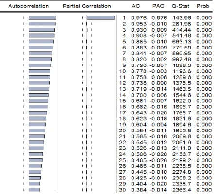
Original CPI data autocorrelations and partial autocorrelations are plotted for the identification. Figure 1 shows the ACF and PACF of the original CPI series. A slowly decaying ACF suggests the non-stationarity of the series. In order to test the stationarity of the series, we used Dickey Fuller unit root test (1979). The results are present in table 1 and it also suggests the non-stationarity of the data.

Table 1. Unit Root Test

t-Statistic Prob.*

Augmented Dickey-Fuller test statistic 2.26076 1.0000

Test critical values: 1% level -3.47647

5% level -2.88169

10% level -2.57759

*MacKinnon (1991) one-sided p- values Figure 1. Correlogram of Original CPI Series

Box-Jenkins suggests differencing of the data, based on the above results. At first difference, the null hypothesis of unit root is rejected which implies data is stationary at first difference i.e. CPI data is integrated of order (1). In order to further smooth the fluctuations, we used simple log of the price. Testing suggests this variable is also non-stationary at level and stationary at first difference. Results of unit root test are present in table 2.

Table 2. Unit Root Test (after difference and log transformation)

t-Statistic Prob.*

Augmented Dickey-Fuller test statistic -15.01822 0.0000

Test critical values: 1% level -3.47614

5% level -2.88154

10% level -2.57751

*MacKinnon (1991) one-sided p- values

After determining the order of integration to make the series stationary, next step is to determine ARMA form of the model. Different orders of AR and MA are used to determine the suitable ARMA structure. The criteria to select the models are Akaike Information Criteria (AIC) and Schwarz Information Criteria (SIC). We performed the test till AR (4) and MA (1). The results are presented in table 3 and 4. Both AIC and SIC suggested the model with the following specification,

Model 1

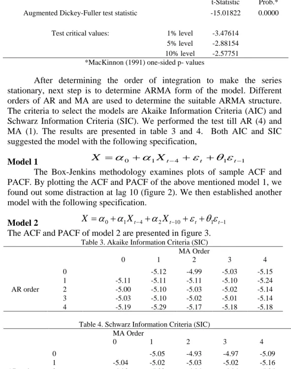
The Box-Jenkins methodology examines plots of sample ACF and PACF. By plotting the ACF and PACF of the above mentioned model 1, we found out some distraction at lag 10 (figure 2). We then established another model with the following specification.

Model 2

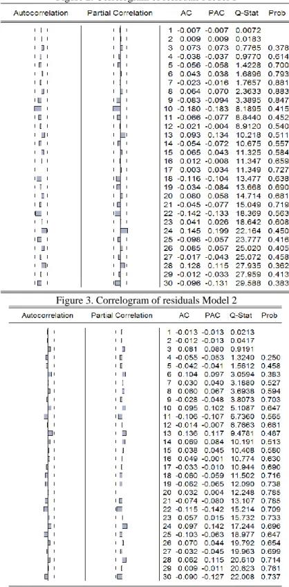
The ACF and PACF of model 2 are presented in figure 3. Table 3. Akaike Information Criteria (SIC)

MA Order 0 1 2 3 4 AR order 0 -5.12 -4.99 -5.03 -5.15 1 -5.11 -5.11 -5.11 -5.10 -5.24 2 -5.00 -5.10 -5.03 -5.02 -5.14 3 -5.03 -5.10 -5.02 -5.01 -5.14 4 -5.19 -5.29 -5.17 -5.18 -5.18

Table 4. Schwarz Information Criteria (SIC) MA Order 0 1 2 3 4 AR order 0 -5.05 -4.93 -4.97 -5.09 1 -5.04 -5.02 -5.03 -5.02 -5.16 2 -4.93 -5.02 -4.94 -4.94 -5.05 3 -4.96 -5.01 -4.93 -4.98 -5.05 4 -5.12 -5.20 -5.09 -5.09 -5.09 1 1 4 1 0 + − + + − = X_{t t t} X

α

α

ε

θ

ε

α

α

α

ε

θ

ε

Figure 2. Correlogram of residuals Model 1

Results

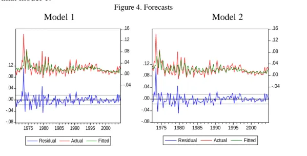
Having selected two ARIMA model specifications we regressed them to get the forecasts to compare the models. Graphical representations of the both the models are presented in figure 4. Seemingly there is not much visible difference between the two forecasts. However, in order to compare further in detail, table 5 presents various comparative statistics such as𝑅2, AIC, SIC, Root Mean Squared Error, Mean Absolute Error, Theil Inequality Coefficient.

The R-square is bit high for the model 2, suggesting it to be a better model. According to AIC model 2 is better than model 1. However, SIC suggests that model 1 is slightly better than model 2. Theil inequality coefficient is used to check the goodness of fit of the forecasted models and the value ranges between 0 and 1, where 0 indicating a perfect fit. In our results according to Theil inequality coefficient model 2 is slightly better than model 1.

Figure 4. Forecasts

Model 1 Model 2

Table 5. Comparative statistics

Model 1 Model 2

R-squared 0.31 0.36

Adjusted R-squared 0.30 0.34 S.E. of regression 0.02 0.02 Durbin-Watson stat 2.01 2.02 Akaike info criterion -5.29 -5.31 Schwarz criterion -5.20 -5.20 Root Mean Squared Error 0.02 0.02 Mean Absolute Error 0.01 0.01 Mean Abs. Percent Error 175.72 167.78 Theil Inequality Coefficient 0.38 0.36

Bias Proportion 0.00 0.00 Variance Proportion 0.58 0.51 Covariance Proportion 0.42 0.49 -.08 -.04 .00 .04 .08 .12 -.04 .00 .04 .08 .12 .16 1975 1980 1985 1990 1995 2000 Residual Actual Fitted

-.08 -.04 .00 .04 .08 .12 -.04 .00 .04 .08 .12 .16 1975 1980 1985 1990 1995 2000 Residual Actual Fitted

Table 6 shows the actual and forecasted values of CPI to further compare the performance of two models. Based on the forecasted errors of the models, model 2 looks better than model 1.

Table 6. Forecast comparison

Quarter Actual CPI Forecast Model 1 Forecast Model 2 Forecast Error Model 1 Forecast Error Model 2 2005Q1 124.34 123.44 123.59 0.90 0.75 2005Q2 127.66 125.74 125.89 1.92 1.77 2005Q3 129.87 129.08 129.24 0.79 0.63 2005Q4 132.09 131.29 131.46 0.80 0.63 2006Q1 134.16 133.51 133.69 0.65 0.47 2006Q2 136.57 135.58 135.76 0.99 0.81 2006Q3 140.82 138.00 138.18 2.82 2.64 2006Q4 143.12 142.27 142.46 0.85 0.66 Conclusion

The study attempts to compare and select an accurate model form various ARIMA models which possess high power of predictability with low error. The study adopted Box-Jenkins approach to forecasting. Various steps are taken in the process, including determining the integration order, model identification and then comparison of the two selected models. The study is based on the quarterly CPI data for Pakistan. Among the two estimated models, which were selected from a number of model specifications, model 2 has come out to be slightly better than model 1. For the purpose of comparison we used the graphical approach first and then we compared the statistics for the two models (e.g. Theil inequality coefficient, AIC). At the end, the actual values of CPI for the quarters of 2005 and 2006 are also compared with the forecasted values. This also turns model 2 to be slightly better.

References:

Brockwell, Peter J., and Richard A. Davis. 2002. Introduction to time series

and forecasting. 2nd ed. Springer texts in statistics. New York: Springer.

Box, G. E. P. and G. M. Jenkins. 1976. Time series analysis: forecasting and

control, Holden-Day.

Callen, Tim, and Dongkoo Chang. 1999. “Modeling and Forecasting

Inflation in India.” IMF Working paper September: 1–36. SSRN:

http://ssrn.com/abstract=880646.

Dickey, David A., and Wayne A. Fuller. 1979. “Distribution of the Estimators for Autoregressive Time Series with a Unit Root.” Journal of the

Diebold, Francis X. 2000. Elements of forecasting. 2nd ed. Cincinnati, Ohio: South-Western College Pub.

Drost, Feike C., Chris A. Klaassen, and Bas J. M. Werker. 1997. “Adaptive estimation in time series models.” Analysis of Statistics 25 (2): 786–817. Fama, Eugene F. 1975. “Short-Term Interest Rates as Predictors of Inflation.” American Economic Review 65 (3): 269-268.

Fama, Eugene F., and Michael R. Gibbons. 1982. “Inflation, Real Returns and Capital Investment.” Journal of Monetary Economics 9 (3): 297–323. MacKinnon, J. G. (1991), “Critical values for cointegration tests,” Chapter

13 in Long-Run Economic Relationships: Readings in Cointegration, ed. R.

F. Engle and C. W. J. Granger. Oxford, Oxford University Press.

Meyler, Aidan, Kenny Geoff, and Terry Quinn. 1998. “Forecasting Irish inflation using ARIMA models.” Central Bank and Financial Services

Authority of Ireland Technical Paper Series 3/RT/98: 1–48.

———. 1998a. “Bayesian VAR Models for Forecasting Irish Inflation.” Central Bank and Financial Services Authority of Ireland Technical Paper

Series 4/RT/98: 1–37.

Salam, Muhammad A., Shazia Salam, and Mete Feridun. 2007. “Modeling and Forecasting Pakistan’s Inflation by Using Time Series ARIMA Models.”

Economic Analysis Working Papers 6: 1–10.

Sekine, Toshitaka. 2001. “Modeling and Forecasting Inflation in Japan.”

IMF Working paper June.

Simone, Francisco N. 2000. “Forecasting Inflation in Chile Using State-Space and Regime-Switching Models.” IMF Working paper Vol: 1–55. SSRN: http://ssrn.com/abstract=880176.

Stockton, David J., and James E. Glassman. 1987. “An Evaluation of the Forecast Performance of Alternative Models of Inflation.” The Review of