BayesX: Analyzing Bayesian Structural Additive Regression Models

September 2005, Volume 14, Issue 11. http://www.jstatsoft.org/

BayesX: Analyzing Bayesian Structured Additive

Regression Models

Andreas Brezger Ludwig-Maximilians-University Munich Thomas Kneib Ludwig-Maximilians-University Munich Stefan Lang University of Leipzig Abstract

There has been much recent interest in Bayesian inference for generalized additive and related models. The increasing popularity of Bayesian methods for these and other model classes is mainly caused by the introduction of Markov chain Monte Carlo (MCMC) simulation techniques which allow realistic modeling of complex problems. This paper de-scribes the capabilities of the free software packageBayesXfor estimating regression models with structured additive predictor based on MCMC inference. The program extends the capabilities of existing software for semiparametric regression included in S-PLUS,SAS,

R or Stata. Many model classes well known from the literature are special cases of the models supported byBayesX. Examples are generalized additive (mixed) models, dynamic models, varying coefficient models, geoadditive models, geographically weighted regression and models for space-time regression. BayesXsupports the most common distributions for the response variable. For univariate responses these are Gaussian, Binomial, Poisson, Gamma, negative Binomial, zero inflated Poisson and zero inflated negative binomial. For multicategorical responses, both multinomial logit and probit models for unordered categories of the response as well as cumulative threshold models for ordered categories can be estimated. Moreover, BayesX allows the estimation of complex continuous time survival and hazard rate models.

Keywords: MCMC, geoadditive models, mixed models, space-time regression, structured ad-ditive regression.

1. Introduction

BayesX is a public domain software package developed during the last eight years at the

pow-erful features and tools for full and empirical Bayesian inference. Functions for handling and manipulating data sets and geographical maps, and for visualizing results are added for convenient use.

In this paper, we describe a powerful tool for estimating regression models with structured additive predictor (see Section2) based on recent MCMC simulation techniques. This paper may primarily serve as a starting point for getting an overview about the capabilities of this tool and as a guideline through the more detailed description in the BayesX manuals (see Brezger, Kneib and Lang 2005). Besides the regression tool described in this paper, the current version of BayesX contains an alternative approach for inference based on mixed model methodology (Fahrmeir, Kneib and Lang 2004;Ruppert, Wand and Carroll 2003), and also allows for estimating graphical models, more specifically Bayesian dags (see Fronk and Giudici 2004;Fronk 2002).

The next two sections provide a brief introduction to the methodological background and a comparison with existing software for comparable models. In Section 4 we give an overview about the general usage of BayesX and show how Bayesian structured additive regression models are estimated. A complex example about childhood undernutrition in Zambia is discussed in Section 5. Instructions for downloading the program and recommendations for further reading are given in the concluding Section6.

2. Methodological background

The model class supported byBayesXis based on the framework of Bayesian generalized linear models (GLM, see Fahrmeir and Tutz 2001). GLMs assume that, given covariates u and unknown parametersγ, the distribution of the response variable y belongs to an exponential family with meanµ=E(y|u, γ) linked to a linear predictorη by

µ=h(η) η=u0γ. (1)

Here h is a known response function, and γ are unknown regression parameters. BayesXis, however, able to estimate much more flexible models with structured additive predictor (see

Brezger and Lang 2005;Fahrmeir, Kneib and Lang 2004)

ηr=f1(xr1) +. . .+fp(xrp) +u0rγ, (2)

where r is a generic observation index, xrj denote generic covariates of different type and

dimension, andfj are (not necessarily smooth) functions of the covariates. The functionsfj

comprise usual nonlinear effects of continuous covariates, time trends and seasonal effects, two-dimensional surfaces, varying coefficient terms, i.i.d. random intercepts and slopes, spa-tially correlated effects, and geographically weighted regression. In order to demonstrate the generality of the model class supported byBayesXwe point out some special cases of (2) well known from the literature:

• Generalized additive model (GAM) for cross-sectional data

A GAM (Hastie and Tibshirani 1990) is obtained if the xj,j= 1, . . . , p, are univariate

and continuous and fj are smooth functions. In BayesX the functions fj are modeled

either by random walk priors or P-splines, see Fahrmeir and Lang (2001a), Lang and Brezger (2004) and Brezger and Lang (2005) for the methodological background.

• Generalized additive mixed model (GAMM)

Consider longitudinal data for individuals i = 1, . . . , n, observed at time points t ∈ {t₁, t2, . . .}. For notational simplicity we assume the same time points for every

indi-vidual, but generalizations to individual-specific time points are obvious. A GAMM extends a GAM by introducing individual-specific random effects, i.e.

ηit=f1(xit1) +. . .+fk(xitk) +b1iwit1+· · ·+bqiwitq+u0itγ,

whereηit, xit1, . . . , xitk, wit1, . . . , witq, uitare predictor and covariate values for individual

iat time tand bi= (b1i, . . . , bqi) is a vector ofq i.i.d. random intercepts (if witj = 1) or

random slopes. The random effects components are modeled by i.i.d. Gaussian priors, see e.g. Clayton (1996). GAMMs can be subsumed into (2) by defining r = (i, t), xrj = xitj, j = 1, . . . , k, xr,k+h = with, and fk+h(xr,k+h) = bhiwith, h = 1, . . . , q.

Similarly, GAMMs for cluster data can be written in the general form (2). • Geoadditive models

In many situations additional geographic information for the observations in the data set is available. As an example compare our demonstrating example in Section 5 on the determinants of childhood undernutrition in Zambia. Here, the district where the mother of a child lives may be used as an indicator for regional differences in the health status of children. A reasonable predictor for such data is

ηr=f1(xr1) +. . .+fk(xrk) +fspat(sr) +u0r, γ (3)

where fspat is an additional spatially correlated effect of the locationsr an observation

pertains to. Models with a predictor that contains a spatial effect are also called geoad-ditive models, see Kammann and Wand (2003). In BayesX, the spatial effect may be modeled by Markov random fields (Besag, York and Molli´e 1991) or two-dimensional P-splines (Brezger and Lang 2005).

• Varying coefficient model (VCM) - geographically weighted regression A VCM as proposed by Hastie and Tibshirani(1993) is defined by

ηr =g1(wr1)zr1+· · ·+gp(wrp)zrp,

where the effect modifierswrj are continuous covariates or time scales and the interacting

variables zrj are either continuous or categorical. This model can be cast into (2) by

xrj = (wrj, zrj) and defining the special function fj(xrj) = fj(wrj, zrj) = gj(wrj)zrj.

Note that inBayesX the effect modifiers are not necessarily restricted to be continuous variables as inHastie and Tibshirani(1993). E.g. the geographical location may be used as effect modifier as well, seeFahrmeir, Lang, Wolff and Bender(2003) for an example. VCM’s with spatially varying regression coefficients are well known in the geography literature as geographically weighted regression, see e.g. Fotheringham, Brunsdon and Charlton(2002).

• ANOVA type interaction model

Supposewr andzr are two continuous covariates. Then, the effect ofwr and zr may be

modeled by a predictor of the form

see e.g. Chen(1993). The functionsf1 andf2 are the main effects of the two covariates

and f1|2 is a dimensional interaction surface which can be modeled e.g. by

two-dimensional P-splines (Lang and Brezger 2004;Brezger and Lang 2005). The interaction can be cast into the form (2) by definingxr1 =wr,xr2 =zr and xr3 = (wr, zr).

All regression models discussed above and arbitrary combinations can be estimated with

BayesXin a Bayesian framework based on recent MCMC simulation techniques. The software

provides a variety of different smoothness priors whose applicability depends on the type of co-variate and the prior assumptions on smoothness. For continuous coco-variates BayesXsupports random walk priors (Fahrmeir and Lang 2001a) and Bayesian P-splines (Lang and Brezger 2004). For spatial effects a variety of Markov random field priors (Besag, York and Molli´e 1991) and two-dimensional P-splines (Brezger and Lang 2005) are available. Unobserved unit-or cluster specific heterogeneity may be considered by introducing random intercepts unit-or slopes. Interactions may be modeled via varying coefficient terms or two-dimensional P-splines. At first sight it may look strange to use one general notation for nonlinear functions of continuous covariates, i.i.d. random intercepts and slopes, and spatially correlated effects as in (2). However, the unified treatment of the different components in our model is justified because the priors for the different types of effects can be cast into a general form. The vector of function evaluationsfj = (fj(x1j), . . . , fj(xnj))0 of an unknown functionfj can be written

as the product of a design matrixXj and a vector of unknown parameters βj, i.e.

fj =Xjβj. (4)

Then, we obtain the predictor (2) in matrix notation as

η=X1β1+· · ·+Xpβp+U γ, (5)

whereU corresponds to the usual design matrix for fixed effects. A prior for a function fj is

now defined by specifying a suitable design matrix Xj and a prior distribution for the vector

βj of unknown parameters. The general form of the prior forβj is

p(βj|τj2)∝exp − 1 2τ2 j β_j0Kjβj ! , (6)

whereKj is a penalty matrix that shrinks parameters towards zero, or penalizes too abrupt

jumps between neighboring parameters. In most cases Kj will be rank deficient and therefore

the prior for βj is partially improper. Specific examples forXj andKj are given inFahrmeir and Lang(2001a),Lang and Brezger(2004) andBrezger and Lang(2005). The general form of the priors allows rather general and unified estimation procedures, see particularlyBrezger and Lang (2005). As a side effect the implementation and description of these procedures is considerably facilitated. The variance parameter τ_j2 in (6) is equivalent to the inverse smoothing parameter in a frequentist approach and controls the trade off between flexibility and smoothness. Weakly informative inverse Gamma hyperpriorτ_j2 ∼IG(aj, bj) are assigned

toτ_j2, withaj =bj = 0.001 as a standard option.

BayesX supports the most common distributions for the response variable. Possible choices

for univariate responses are Gaussian, Binomial, Poisson, Gamma, negative Binomial, zero inflated poisson and zero inflated negative binomial. For multicategorical responses, both

multinomial logit and probit models for unordered categories of the response as well as cumu-lative threshold models for ordered categories are available. Note that models for categorical responses may also be used for estimating discrete time survival and competing risk models, seeFahrmeir and Tutz(2001), Ch. 9. The Poisson distribution allows the estimation of piece-wise exponential survival models, see e.g. Ibrahim, Chen and Sinha (2001). Furthermore, extensions of continuous time Cox models have been added toBayesXrecently.

The goodness of fit is assessed by the deviance, deviance residuals, the deviance information criterion DIC (Spiegelhalter, Best, Carlin and van der Linde 2002) and leverage statistics. The methodology for univariate responses is described in full detail in Fahrmeir and Lang

(2001a), Lang and Brezger (2004) and Brezger and Lang (2005). Count data regression is covered inFahrmeir and Osuna(2003). Models with multicategorical responses are dealt with inFahrmeir and Lang(2001b) and Brezger and Lang (2005). Survival models are treated in

Hennerfeind, Brezger and Fahrmeir(2005) andFahrmeir and Hennerfeind(2003). A thorough (and for most practical purposes sufficient) introduction into the regression models supported by the program is provided in theBayesXmethodology manual.

3. Comparison with existing software

This section compares the capabilities of BayesXto estimate (subclasses of) structured addi-tive regression models with other statistical software packages.

3.1. Software with built-in functions

We first compare the functionality of BayesXwith that of other statistical software packages with built in functions for additive or related models. The comparison includes the step.gam function in S-PLUS (Insightful Corporation 2003), the packages mgcv, polspline, geoR and fieldsinR(RDevelopment Core Team 2004), theSAS-proceduresgam,loess,tpspline,krige2d and mixed(SAS Institute Inc. 2004), and the functions gamand gllamm, which are available for usage inStata(StataCorp. 2003). It turns out that BayesXextends the standard software in several ways and therefore provides a more flexible tool for complex regression analysis. Table 4 gives a summary of the different model terms supported by BayesX. Most of the competing implementations support either additive models, possibly including interaction surfaces, or the possibility to estimate spatial effects, mostly based on geostatistical method-ology. However, none of them supports all combinations of additive and spatial components implemented inBayesX. In addition,BayesXallows for random effects, which are only available in two other programs, and further extensions such as seasonal priors and varying coefficient terms, which are not implemented in any other software included in the comparison.

Another issue is the class of response distributions supported by the different programs. Table 2 lists these distributions separately for univariate responses, categorical responses and survival models. While most of the implementations support univariate responses, only a limited number allows for the extended model classes supported by BayesX. The most competitive implementation is thegllammfunction inStata, which, however, does not include most of the model terms of structured additive regression models. Similarly, the polspline package in Rallows for nominal categorical responses and continuous time survival analysis, but does not support the inclusion of spatial or random effects.

n on p ar amet ri c ter ms (e. g. P -sp li n es) in ter act ion su rf aces sp at ial ter ms (sp at ial h et er o-gen ei ty ) ran d om effect s season al p ri or s v ar y in g co effi-ci en ts B a yesX • • • • • • S -P L U S ste p .gam • ◦ ◦ ◦ ◦ ◦ R mgcv • • ◦ • ◦ ◦ p ol sp li n e • • ◦ ◦ ◦ ◦ ge oR / ge oR gl m ◦ ◦ • ◦ ◦ ◦ fi e ld s ? ? ? ◦ ◦ ◦ S A S pro c gam • • ◦ ◦ ◦ ◦ p ro c lo e ss ? ? ◦ ◦ ◦ ◦ p ro c tp sp li n e ? ? ◦ ◦ ◦ ◦ p ro c k ri ge 2d ◦ ◦ • ◦ ◦ ◦ p ro c mi x e d ◦ ◦ • • ◦ ◦ S ta ta gam • ◦ ◦ ◦ ◦ ◦ gl lamm ◦ ◦ ◦ • ◦ ◦ • a v ai lab le ◦ n ot a v ai lab le ? on ly on e of th e mo d el ter ms can b e u sed T ab le 1: S u p p or ted mo d el ter ms in B a yesX an d comp et in g sof tw ar e.

u n iv ar iat e resp on ses cat egor ical resp on ses su rv iv al mo d el s B a yesX G au ssi an , b in omi al , p oi sson , gamma, n eg-at iv e b in omi al , zer o in fl at ed p oi sson , zer o in fl at ed n egat iv e b in omi al m u lt in omi al logi t an d p ro-b it , cu m u lat iv e p rob it h azar d regr essi on S -P L U S ste p .gam G au ssi an , b in omi al , p oi sson , gamma x x R mgcv G au ssi an , b in omi al , p oi sson , gamma, n eg-at iv e G au ssi an , n egat iv e b in omi al x x p ol sp li n e x m u lt in omi al logi t h azar d regr essi on ge oR / ge oR gl m G au ssi an , b in omi al , p oi sson x x fi e ld s G au ssi an S A S pro c gam G au ssi an , b in omi al , p oi sson , gamma, in -v er se G au ssi an x x p ro c lo e ss G au ssi an x x p ro c tp sp li n e G au ssi an x x p ro c k ri ge 2d G au ssi an x x p ro c mi x e d G au ssi an x x S ta ta gam G au ssi an , b in omi al , p oi sson , gamma x Co x mo d el gl lamm G au ssi an , b in omi al , p oi sson , gamma m u lt in omi al logi t, cu m u la-ti v e logi t an d p rob it x T ab le 2: S u p p or ted resp on se d ist ri b u ti on s in B a yesX an d comp et in g sof tw ar e.

3.2. Comparison with WinBUGS

Currently, the most widely used software for Bayesian inference isWinBUGS (Spiegelhalter, Thomas, Best and Lunn 2003) which has been developed by the MRC Biostatistics Unit in Cambridge. The package is available free of charge at http://www.mrc-bsu.cam.ac. uk/bugs/. WinBUGS may be seen as a kind of (easy to use) programming language that allows to specify and estimate almost any Bayesian model. Hence, in principle the models supported in BayesX could be estimated in WinBUGS as well. However, a price is payed for the extreme flexibility: Our comparison with WinBUGSshows thatBayesXis much faster and

−3 −2 −1 0 1 2 3 −1.5 −0.5 0.5 1.5 covariate

BayesX

−3 −2 −1 0 1 2 3 −1.5 −0.5 0.5 1.5 covariate

WinBUGS (tps)

−3 −2 −1 0 1 2 3 −1.5 −0.5 0.5 1.5 covariate

WinBUGS (MM)

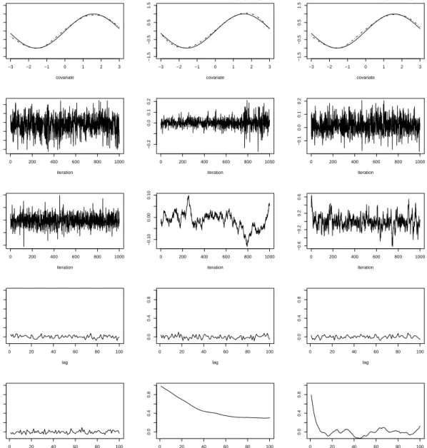
0 200 400 600 800 1000 −1.5 −0.5 0.5 iteration 0 200 400 600 800 1000 −0.2 0.0 0.1 0.2 iteration 0 200 400 600 800 1000 −0.1 0.0 0.1 0.2 iteration 0 200 400 600 800 1000 −2 −1 0 1 2 iteration 0 200 400 600 800 1000 −0.10 0.00 0.10 iteration 0 200 400 600 800 1000 −0.6 −0.2 0.2 0.6 iteration 0 20 40 60 80 100 0.0 0.4 0.8 lag 0 20 40 60 80 100 0.0 0.4 0.8 lag 0 20 40 60 80 100 0.0 0.4 0.8 lag 0 20 40 60 80 100 0.0 0.4 0.8 lag 0 20 40 60 80 100 0.0 0.4 0.8 lag 0 20 40 60 80 100 0.0 0.4 0.8 lag

Figure 1: Estimation (top), selected sampling paths and corresponding autocorrelations (Gaussian response, 6000 iterations, 1000 burn-in, step 5).

Response N BayesX WinBUGS (tps) WinBUGS (MM) Gaussian 200 <5 sec. ca. 5 min. ca. 5 min. Bernoulli 500 <20 sec. ca. 76 min. ca. 92 min. Table 3: Simulation run time on a PC (0.99GB RAM, 2.79GHz CPU).

−3 −2 −1 0 1 2 3 −1.5 −0.5 0.5 1.5 covariate

BayesX

−3 −2 −1 0 1 2 3 −1.5 −0.5 0.5 1.5 covariate

WinBUGS (tps)

−3 −2 −1 0 1 2 3 −1.5 −0.5 0.5 1.5 covariate

WinBUGS (MM)

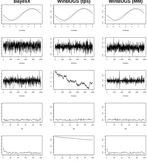
0 200 400 600 800 1000 −1.4 −1.0 −0.6 −0.2 iteration 0 200 400 600 800 1000 −0.4 0.0 0.2 0.4 iteration 0 200 400 600 800 1000 −0.4 0.0 0.2 0.4 iteration 0 200 400 600 800 1000 −1 0 1 2 3 iteration 0 200 400 600 800 1000 −4 −3 −2 −1 iteration 0 200 400 600 800 1000 −0.5 0.0 0.5 iteration 0 20 40 60 80 100 0.0 0.4 0.8 lag 0 20 40 60 80 100 0.0 0.4 0.8 lag 0 20 40 60 80 100 0.0 0.4 0.8 lag 0 20 40 60 80 100 0.0 0.4 0.8 lag 0 20 40 60 80 100 0.0 0.4 0.8 lag 0 20 40 60 80 100 0.0 0.4 0.8 lag

Figure 2: Estimation, selected sampling paths and corresponding autocorrelations (Bernoulli response, 12000 iterations, 2 burnin, step 10).

shows superior mixing properties for the resulting Markov chains.

We demonstrate the differences with two simple examples. The two models yi ∼N(sin(xi),0.5), i= 1, . . . ,200 and yi ∼B(1, πi), πi= exp(sin(xi) 1 + exp(sin(xi)) i= 1, . . . ,500

have been estimated both with BayesX and WinBUGS using Bayesian P-splines with second order random walk penalty. InWinBUGSboth the truncated power series basis (tps) of splines as well as a mixed model representation (MM) have been tested. Table 3 shows thatBayesX

estimates the models roughly 60-280 times faster than WinBUGS. Moreover, the MCMC sampler of BayesX shows considerably improved mixing properties compared to WinBUGS, see Figures1 and2. The resulting estimators are, however, quite close.

4. Usage of

BayesX

After having started BayesX, a main window divided into four sub-windows appears on the screen. These are a command window for entering and executing code, anoutput windowfor displaying results, areview window for easy access to past commands, and anobject browser that displays all objects currently available.

BayesX is object oriented although the concept is limited, i.e. inheritance and other concepts

of object oriented languages like C++ or S-PLUS are not supported. For every object type a number of object-specific methods may be applied to a particular object. To estimate Bayesian regression models we need a dataset object to incorporate, handle and manipulate data, a bayesreg object to estimate semiparametric regression models, and agraph object to visualize estimation results. If spatial effects are to be estimated, we additionally need a map object. map objectsmainly serve as auxiliary objects for bayesreg objectsand are used to read the boundary information of geographical maps and to compute the neighborhood matrix and weights associated with the neighbors. The syntax for generating a new object in BayesXis > objecttype objectname

where objecttype is the type of the object, e.g. dataset, and objectname is the arbitrarily chosen name of the new object. In the following subsections we give an overview about the most important methods of the object types required to estimate Bayesian structured additive regression models.

4.1. dataset objects

Data (in form of external ASCII files) are read into BayesXwith the infile command. The general syntax is:

> objectname.infile[varlist] [,options]usingfilename

Here,varlistdenotes a list of variable names separated by blanks (or tabs), andfilenameis the name (including full path) of the external ASCII file storing the data. The variable list may be omitted if the first line of the file already contains the variable names. BayesX assumes

that the variables are stored column wise, that is one column per variable. Two options may be passed, themissing option to indicate missing values and the maxobs option for reading in large data sets. Specifying for example ’missing = M’ defines the letter ’M’ as an indicator for a missing value. The default values are a period ’.’ or ’NA’ (which remain valid indicators for missing values even if an additional indicator is defined). Themaxobsoption may be used to speed up the reading of large data sets. Its usage is strongly recommended if the number of observations exceeds 10000. For instance, ’maxobs=100000’ indicates that the data set has 100000 or less observations. Having read in the data, the data set may be inspected by double clicking on the respective object in theobject browser.

Besides theinfile command many more methods for handling and manipulating data are available, e.g. thegenerate command to create new variables, the drop command to drop observations and variables or the descriptive command to obtain summary statistics for the variables.

4.2. map objects

The boundary information of a geographical map is read into BayesXusing the infile com-mand of map objects. The current version supports two file formats,boundary filesandgraph files. Aboundary filestores the boundaries of every region in form of closed polygons. Having read in a boundary file,BayesXautomatically computes the neighbors and associated weights of each region. By double clicking on the respective object in the object browser the map may be inspected visually. A graph file simply stores the nodes N and edges E of a graph G= (N, E), which is a convenient way of representing the neighborhood structure of a geo-graphical map. The nodes of the graph correspond to the region codes. The neighborhood structure is represented by the edges of the graph. Weights associated with the edges may be given in a graph file as well. For the detailed structure of boundaryand graph fileswe refer to theBayesX reference manual, Ch. 5. Examples of boundary and graph files for different countries and regions are available at the BayesX homepage, see Section 6 for the internet address. The syntax for reading boundary or graph files is

> objectname.infile[, weightdef=wd] [graph]usingfilename

where option weigthdef specifies how the weights associated with each pair of neighbors are computed. Currently, there are three weight specifications available, ’weightdef=adjacency’, ’weightdef=centroid’ and ’weightdef=combnd’. If ’weightdef=adjacency’ is specified, the weights for each pair of neighbors are set equal to one. Specifying ’weightdef=centroid’ results in weights inverse proportional to the distance of the centroids of neighboring regions and ’weightdef=combnd’ results in weights proportional to the length of the common bound-ary. If ’graph’ is specified as an additional option BayesXexpects a graph file rather than a boundary file.

4.3. bayesreg objects

Bayesian regression models are estimated using the regress command of bayesreg objects. The general syntax is

> objectname.regressmodel[weightweightvar] [if expression] [,options]usingdataset Executing this command estimates the regression model specified in model using the data

specified indataset, where dataset is the name of adataset object created previously. An if statement may be included to analyze only a part of the data and a weight variableweightvar to estimate weighted regression models. Options may be passed to specify the response distribution, details of the MCMC algorithm (for example the number of iterations or the thinning parameter), etc. The syntax of models is:

depvar=term1 +term2 + · · ·+termr

Here,depvar specifies the dependent variable in the model and term1, . . . , termr define the

way the covariates influence the response variable. The different terms must be separated by ’+’ signs. In the following we give some examples. An overview about the capabilities of

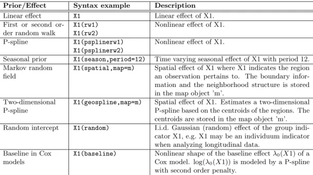
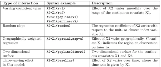
BayesXis given in Table 4. Table 5 shows how interactions between covariates are specified.

More details can be found in theBayesXmanual Ch. 7.

Suppose we want to model the effect of three covariates X1, X2 and X3 on the response variable Y. Traditionally a strictly linear predictor is assumed which can be specified inBayesXby: Y = X1 + X2 + X3

Note that a constant intercept is automatically included into the models and must not be specified. If we assume possibly nonlinear effects of the continuous variables X1 and X2, for instance quadratic P-splines with second order random walk smoothness priors, we obtain: Y = X1(psplinerw2,degree=2) + X2(psplinerw2,degree=2) + X3

The second argument in the model formula above is optional. If omitted, a cubic spline will be estimated by default. Moreover, some more optional arguments may be passed, e.g. to define the number of knots. For details we refer to theBayesXmanual.

Prior/Effect Syntax example Description

Linear effect X1 Linear effect of X1. First or second

or-der random walk

X1(rw1) X1(rw2) Nonlinear effect of X1. P-spline X1(psplinerw1) X1(psplinerw2) Nonlinear effect of X1.

Seasonal prior X1(season,period=12) Time varying seasonal effect of X1 with period 12. Markov random

field

X1(spatial,map=m) Spatial effect of X1 where X1 indicates the region an observation pertains to. The boundary infor-mation and the neighborhood structure is stored in the map object ’m’.

Two-dimensional P-spline

X1(geospline,map=m) Spatial effect of X1. Estimates a two-dimensional P-spline based on the centroids of the regions. The centroids are stored in the map object ’m’. Random intercept X1(random) I.i.d. Gaussian (random) effect of the group

indi-cator X1, e.g. X1 may be an individuum indiindi-cator when analyzing longitudinal data.

Baseline in Cox models

X1(baseline) Nonlinear shape of the baseline effectλ0(X1) of a

Cox model. log(λ0(X1)) is modeled by a P-spline

with second order penalty.

Type of interaction Syntax example Description

Varying coefficient term X2*X1(rw1) X2*X1(rw2) X2*X1(psplinerw1) X2*X1(psplinerw2)

Effect of X2 varies smoothly over the range of the continuous covariate X1. Random slope X2*X1(random) The regression coefficient of X2 varies with

respect to the unit- or cluster index vari-able X1.

Geographically weighted regression

X2*X1(spatial,map=m) Effect of X2 varies geographically. Covari-ate X1 indicCovari-ates the region an observation pertains to.

Two-dimensional surface

X2*X1(pspline2dimrw1) Two-dimensional surface for the continu-ous covariates X1 and X2.

Time-varying effect in Cox models

X2*X1(baseline) Effect of X2 varies over time, where the time-axis is given by X1

Table 5: Possible interaction terms in BayesX.

Family Link Description

gaussian identity Gaussian responses. Details about MCMC inference in Lang and Brezger(2004).

binomial logit Binomial responses. Inference is based on conditional prior or IWLS proposals, see Fahrmeir and Lang (2001a) and Brezger and Lang

(2005).

bernoullilogit logit Models with binary responses and logit link. Estimation is based on latent utility representations, seeHolmes and Held(2004).

binomialprobit probit Models with binary responses and probit link. Estimation is based on latent utility representations, seeAlbert and Chib(1993).

multinomial logit Multinomial logit model, seeBrezger and Lang(2005).

multinomialprobit probit Multinomial probit model. Estimation is based on latent utility rep-resentations, seeFahrmeir and Lang(2001b).

cumprobit probit Cumulative threshold model for ordered responses with three cat-egories. Estimation is based on latent utility representations, see

Fahrmeir and Lang(2001b).

poisson log Poisson distribution. Inference is based on conditional prior or IWLS proposals, see Fahrmeir and Lang (2001a) and Brezger and Lang

(2005).

negbin log Negative Binomial responses. Details inFahrmeir and Osuna(2003). gamma log Gamma distribution. Inference is based on conditional prior or IWLS proposals, see Fahrmeir and Lang (2001a) and Brezger and Lang

(2005).

zip log Zero inflated count data regression.

cox – Cox model. Details inHennerfeind, Brezger and Fahrmeir(2005) and

Fahrmeir and Hennerfeind(2003).

Suppose now that we observe an additional variable L which provides information about the geographical location an observation pertains to. A spatial effect based on a Markov random field prior is added by:

Y = X1(psplinerw2,degree=2) + X2(psplinerw2,degree=2) + X3 + L(spatial,map=m) The option mapspecifies the map object that contains the boundaries of the regions and the neighborhood information required to estimate a spatial effect.

The distribution of the response is specified by adding the option family to the options list. For instance, ’family=gaussian’ defines the responses to be Gaussian. Other valid specifications are found in Table 6.

4.4. graph objects

graph objects are used to visualize data and estimation results obtained by other objects in

BayesX. Currentlygraph objectsmay be used to draw scatter plots between variables (method

plot), or to draw and color geographical maps stored inmap objects (methoddrawmap). We illustrate the usage ofgraph objectswith method drawmap which is used to color the regions of a map according to some numerical characteristics. The syntax is:

> objectname.drawmap plotvar regionvar[if expression] ,map=mapname[options]using dataset

Method drawmap draws the map stored in the map object mapname and prints the graph either on the screen or stores it as a postscript file (if option outfile is specified). The regions with region coderegionvarare colored according to the values of the variableplotvar. The variablesplotvar and regionvar are supposed to be stored in the dataset object dataset. Several options are available for customizing the graph, e.g. for changing from grey scale to color scale or storing the map as a postscript file, see theBayesX reference manual Ch. 6. A typical graph obtained with methoddrawmap is given in Figure 4.

5. A complex example: Childhood undernutrition in Zambia

In this example we demonstrate the usage of BayesXby analyzing data on undernutrition of children in Zambia. This data set has already been analyzed in Kandala, Lang, Klasen and Fahrmeir(2001). Here, we apply the same model as developed in their paper. Since our focus is on demonstrating how a regression model can be specified and estimated usingBayesXwe do not discuss or interpret the estimation results.

Undernutrition among children is usually determined by assessing the anthropometric status of a child relative to a reference standard. In our example undernutrition is measured through stunting or insufficient height for age, indicating chronic undernutrition. Stunting for a child iis determined using a Z-score defined as

Zi =

AIi−MAI

σ ,

where AI refers to the child‘s anthropometric indicator (height at a certain age in our ex-ample), MAI refers to the median of the reference population and σ refers to the standard deviation of the reference population.

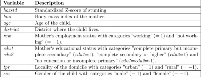
Variable Description

hazstd Standardized Z-score of stunting. bmi Body mass index of the mother. agc Age of the child.

district District where the child lives.

rcw Mother‘s employment status with categories ”working” (= 1) and ”not work-ing” (= −1).

edu1 edu2

Mother‘s educational status with categories ”complete primary but incom-plete secondary” (edu1=1), ”comincom-plete secondary or higher” (edu2=1) and ”no education or incomplete primary” (edu1=edu2=-1).

tpr Locality of the domicile with categories ”urban” (= 1) and ”rural” (= −1). sex Gender of the child with categories ”male” (= 1) and ”female” (=−1).

Table 7: Variables in the data set on childhood undernutrition.

The main interest is on modeling the dependence of undernutrition on covariates including the age of the child, the body mass index of the child‘s mother, the district the child lives in and some further categorical covariates. Table7 gives a description of the variables used in our model.

The data is analyzed in largely five steps: We first read in the data intoBayesXusing adataset object. Since we want to estimate a spatial effect of the district in which the child lives, we need the boundaries of the districts to compute the neighborhood information of the map of Zambia. Therefore, we create a map object which contains the required information in the second step. A regression model is estimated in the third step followed by visualizing results. Since our analysis is based on MCMC techniques it is important to investigate the sampling paths and the autocorrelation functions of the estimated parameters in a last step.

In the following, we assume that the data set and the map of Zambia are stored in the files c:\data\zambia.rawand c:\data\mapzambia.raw, respectively.

1. Reading data set information

To read the data into BayesX, we create a dataset object and use the infile command of dataset objects:

> dataset d

> d.infile using c:\data\zambia.raw

2. Compute neighborhood information

The neighborhood information of the map of Zambia is computed and stored in BayesX by creating amap object and using theinfile command:

> map m

> m.infile using c:\data\mapzambia.raw

matrix of the map. In our example, two regions are assumed to be neighbors if they share a common boundary.

3. Regression analysis

Kandala, Lang, Klasen and Fahrmeir (2001) estimated a Gaussian regression model with predictor

η = γ0+γ1rcw+γ2edu1 +γ3edu2 +γ4tpr+γ5sex +f1(bmi) +f2(agc)+

fstr(district) +funstr(district)

(7) The two continuous covariates bmi and agc are assumed to have a possibly nonlinear effect on the Z-score and are therefore modeled nonparametrically (as cubic P-splines with second order random walk prior in our example). The spatial effect of the district is split up into a spatially correlated partfstr(district) and an uncorrelated partfunstr(district). The former is

modeled by a Markov random field prior, where the neighborhood matrix and possible weights associated with the neighbors are obtained from themap objectm. The latter is modeled by an i.i.d. Gaussian effect.

We now estimate model (7) using bayesreg objects. We create abayesreg object and estimate the model using the regress command:

> bayesreg b

> b.regress hazstd = rcw + edu1 + edu2 + tpr + sex + bmi(psplinerw2) + agc(psplinerw2) + district(spatial,map=m) + district(random), family=gaussian iterations=12000 burnin=2000 step=10 predict using d

The optionsiterations,burninandstepdefine the number of iterations, the burn in period and the thinning parameter of the MCMC simulation run. Specifyingstep=10as above forces

BayesXto store only every 10th sampled parameter which leads to a random sample of length

1000 for every parameter in our example.

If option predict is specified, samples of the deviance, the effective number of parameters pD and the deviance information criterion DIC of the model are computed and stored, see Spiegelhalter, Best, Carlin and van der Linde(2002). In addition, estimates for the additive predictor and the posterior expectations are computed for every observation.

On a 2.4 GHz personal computer estimation of the model is carried out in about 1 minute and 5 seconds.

After estimation, results for each effect are written to an external ASCII file. These files contain the posterior mean and median, the posterior 2.5%, 10%, 90% and 97.5% quantiles and the corresponding 95% and 80% posterior probabilities of the estimated effects. For example, the beginning of the file for the effect ofbmilooks like this:

intnr bmi pmean pqu2p5 pqu10 pmed pqu90 pqu97p5 pcat95 pcat80

1 12.8 -0.284065 -0.660801 -0.51678 -0.283909 -0.0585753 0.085998 0 -1 2 13.15 -0.276772 -0.609989 -0.483848 -0.275156 -0.070517 0.0572406 0 -1 3 14.01 -0.258674 -0.515628 -0.416837 -0.257793 -0.10009 -0.00289024 -1 -1

The numbers1 and-1 for the variables pcat95 and pcat80 indicate that the corresponding credible intervals are either strictly positive or negative. Zero indicates credible intervals containing zero.

4. Visualizing estimation results

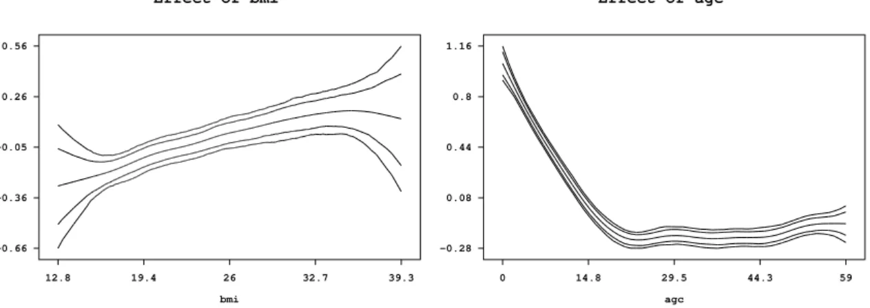
Estimation results for nonlinear effects ofbmi and agc and the spatial effect of the district are best summarized by visualization. BayesXautomatically creates appropriate plots of the effects and stores the graphs as postscript files. The file names are given in theoutput window for each effect. Figure3and Figure4show the content of these files. Moreover, a batch-file is created that contains all commands necessary to reproduce the plots. The advantage is that additional options may be added by the user to customize the graphs (e.g. to change the title or axis labels).

It is also possible to visualize effects on the screen immediately after estimation. For the nonlinear effects of the two continuous covariates such plots are obtained by executing the

12.8 19.4 26 32.7 39.3 -0.66 -0.36 -0.05 0.26 0.56 Effect of bmi bmi 0 14.8 29.5 44.3 59 -0.28 0.08 0.44 0.8 1.16 Effect of agc agc

Figure 3: Example on childhood undernutrition: Effect of the body mass index of the child‘s mother and of the age of the child together with pointwise 80% and 95% credible intervals.

-0.304985 0 0.22614

commands > b.plotnonp 1 and

> b.plotnonp 3

The numbers following theplotnonpcommand depend on the order in which the model terms have been specified. They are supplied in theoutput windowafter estimation.

Results for spatial effects are best visualized by drawing the respective map and coloring the regions of the map according to some characteristic of the posterior, e.g. the posterior mean. For instance, the structured spatial effect is visualized by typing

> b.drawmap 5, color

The additional optioncolor forcesBayesXto use colors instead of grey shades for visualiza-tion.

5. Post estimation commands

In addition to the regress command, bayesreg objects provide some post estimation com-mands to get sampled parameters or to compute autocorrelation functions of sampled param-eters. For example

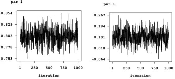
> b.getsample

stores sampled parameters in ASCII files and plots the sampling paths. The resulting graphs are stored in postscript format leading e.g. to the plots shown in Figure 5 for the scale parameter and the intercept. To avoid too large files, the samples are typically partitioned into several files.

Autocorrelation functions may be drawn e.g. by typing

1 250 500 750 1000 0.753 0.778 0.803 0.829 0.854 iteration par 1 1 250 500 750 1000 -0.064 0.018 0.101 0.184 0.267 iteration par 1

Figure 5: Example on childhood undernutrition: Sampling paths for the scale parameter and the intercept.

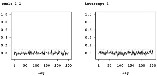
1 50 100 150 200 250 0.0 0.2 0.4 0.6 0.8 1.0 lag scale_1_1 1 50 100 150 200 250 0.0 0.2 0.4 0.6 0.8 1.0 lag intercept_1

Figure 6: Example on childhood undernutrition: Autocorrelation functions for the scale parameter and the intercept.

> b.plotautocor , maxlag=150

wheremaxlagspecifies the maximum lag number. The default is ’maxlag=250’. Executing the plotautocor command also stores the autocorrelation functions in an ASCII file. Figure 6

shows the autocorrelation function for the scale parameter and the intercept.

6. Download and recommendations for further reading

The latest version of BayesX including detailed manuals is available at http://www.stat. uni-muenchen.de/~bayesx/.

TheBayesXhomepage also contains all files required to reproduce the results presented in the

example on childhood undernutrition in Zambia. In addition, a more detailed tutorial based on the Zambia data set is available, click onTutorialsat the homepage. Finally, to download the boundary and graph files for a number of countries and regions, click onMaps.

For users not familiar with MCMC simulation techniques, it is strongly recommended to read at least one of the introductions into MCMC. A very nice and thorough introduction is given inGreen(2001). To get an overview about the methodologyBayesXis based on, we consider it sufficient to read the methodology manual. More details may be found in the references cited therein and in this paper. First steps withBayesXcan be done with the example of this paper and the tutorial on childhood undernutrition in Zambia.

Acknowledgements

We thank Ludwig Fahrmeir, Eva-Maria Fronk and Andrea Hennerfeind for helpful comments and discussions. This research has been financially supported by grants from the German Sci-ence Foundation (DFG), Collaborative Research Center 386 ”Statistical Analysis of Discrete Structures”.

References

Albert J, Chib S (1993). ”Bayesian Analysis of Binary and Polychotomous Response Data.” Journal of the American Statistical Association,88, 669–679.

Besag J, York J, Molli´e A (1991). ”Bayesian Image Restoration with two Applications in Spatial Statistics (with discussion).”Annals of the Institute of Statistical Mathematics,43, 1–59.

Brezger A, Kneib T, Lang S (2005). BayesX Manuals, Ludwig-Maximilians-University, Mu-nich, URLhttp://www.stat.uni-muenchen.de/~bayesx/.

Brezger A, Lang S (2005). ”Generalized Structured Additive Regression Based on Bayesian P-splines.”Computational Statistics and Data Analysis, in press. Preprint available athttp: //www.stat.uni-muenchen.de/sfb386/papers/dsp/paper321.pdf

Chen Z (1993). ”Fitting Multivariate Regression Functions by Interaction Spline Models.” Journal of the Royal Statistical Society B,55, 473–491.

Clayton D (1996). ”Generalized Linear Mixed Models.” In: Gilks WR, Richardson S, Spiegel-halter DJ:”Markov Chain Monte Carlo in Practice.”Chapman and Hall, London.

Fahrmeir L, Hennerfeind A (2003). ”Nonparametric Bayesian Hazard Rate Models Based on Penalized Splines.” SFB 386 Discussion paper 361, University of Munich. Available at

http://www.stat.uni-muenchen.de/sfb386/papers/dsp/paper361.ps

Fahrmeir L, Kneib T, Lang S (2004). ”Penalized Structured Additive Regression for Space-Time Data: A Bayesian Perspective.”Statistica Sinica,14, 731–761.

Fahrmeir L, Lang S (2001a). ”Bayesian Inference for Generalized Additive Mixed Models Based on Markov Random Field Priors.”Journal of the Royal Statistical Society C, 50, 201–220.

Fahrmeir L, Lang S (2001b) ”Bayesian Semiparametric Regression Analysis of Multicategorical Time-Space Data.”Annals of the Institute of Statistical Mathematics,53, 10–30.

Fahrmeir L, Lang S, Wolff J, Bender S (2003). ”Semiparametric Bayesian Time-Space Analysis of Unemployment Duration.”Journal of the German Statistical Society,87, 281–307. Fahrmeir L, Osuna L (2003). ”Structured Count Data Regression.” SFB 386 Discussion

pa-per 334, University of Munich. Available athttp://www.stat.uni-muenchen.de/sfb386/ papers/dsp/paper334.ps

Fahrmeir L, Tutz G (2001) Multivariate Statistical Modelling Based on Generalized Linear Models. Springer, New York.

Fotheringham AS, Brunsdon C, Charlton ME (2002). Geographically Weighted Regression: The Analysis of Spatially Varying Relationships.Chichester, Wiley.

Fronk EM (2002). ”Model Selection for Dags via RJMCMC for the Discrete and Mixed Case.” SFB 386 Discussion Paper 271, Department of Statistics, University of Munich. Available athttp://www.stat.uni-muenchen.de/sfb386/papers/dsp/paper271.ps

Fronk EM, Giudici P (2004). ”Markov Chain Monte Carlo Model Selection for Dag Models.” Statistical Methods and Application,13, 259–273.

Green PJ (2001). ”A Primer in Markov Chain Monte Carlo.” In: Barndorff-Nielsen OE, Cox DR, Kl¨uppelberg C (eds.).Complex Stochastic Systems. Chapmann and Hall, London. Hastie T, Tibshirani R (1990).Generalized Additive Models. Chapman and Hall, London. Hastie T, Tibshirani R (1993). ”Varying-Coefficient Models.”Journal of the Royal Statistical

Society B,55, 757–796.

Hennerfeind A, Brezger A, Fahrmeir L (2005) ”Geoadditive Survival Models.” SFB Discussion paper 414, University of Munich. Revised for Journal of the American Statistical Asso-ciation. Preprint available at http://www.stat.uni-muenchen.de/sfb386/papers/dsp/ paper414.pdf

Holmes CC, Held L (2006) ”Bayesian Auxiliary Variable Models for Binary and Multinomial Regression.”Bayesian Statistics,1, 145–168.

Ibrahim JG, Chen MH, Sinha D (2001).Bayesian Survival Analysis. Springer, New YorK. Kamman EE, Wand MP (2003). ”Geoadditive Models.”Journal of the Royal Statistical Society

C,52, 1–18.

Kandala NB, Lang S, Klasen S, Fahrmeir L (2001). ”Semiparametric Analysis of the Socio-Demographic and Spatial Determinants of Undernutrition in Two African Countries.” Re-search in Official Statistics,1, 81–100.

Lang S, Brezger A (2004). ”Bayesian P-Splines.”Journal of Computational and Graphical Statistics,13, 183–212.

RDevelopment Core Team (2004).R: A Language and Environment for Statistical Computing,

R Foundation for Statistical Computing, Vienna, Austria. URL http://www.R-project. org/.

Ruppert D, Wand MP, Carroll RJ (2003).Semiparametric Regression. Cambridge University Press.

SAS Institute Inc. (2004).SAS/STATsoftware, Version 8, Cary, NC. URLhttp://www.sas. com/.

Spiegelhalter DJ, Best NG, Carlin BP, van der Linde A (2002). ”Bayesian Measures of Model Complexity and Fit.”Journal of the Royal Statistical Society B, 65, 583–639.

Spiegelhalter D, Thomas A, Best N, Lunn D (2003).WinBUGS User Manual (Version 1.4). Medical Research Council Biostatistics Unit, Cambridge, UK, URLhttp://www.mrc-bsu. cam.ac.uk/bugs/.

Insightful Corporation (2003). S-PLUS (Version 6.2), Seattle, WA, URL http://www. insightful.com/.

StataCorp. (2003).StataStatistical Software: Release 8. College Station, TX: StataCorp LP. URLhttp://www.stata.com/.

Affiliation:

Andreas Brezger, Thomas Kneib Department of Statistics

Ludwigstraße 33

Ludwig-Maximilians-University Munich 80539 M¨unchen, Germany

Stefan Lang

Institute of Empirical Economic Research Marschnerstraße 31

University of Leipzig 04109 Leipzig, Germany

E-mail: [email protected]

URL:http://www.stat.uni-muenchen.de/~bayesx/

Journal of Statistical Software

Submitted: 2004-06-18 September 2005, Volume 14, Issue 11. Accepted: 2005-09-09