Efficient Bayesian inference for COM-Poisson regression models

DOI 10.1007/s11222-017-9750-x

Efficient Bayesian inference for COM-Poisson regression models

Agostino Nobile2

Received: 15 November 2016 / Accepted: 18 April 2017 © The Author(s) 2017. This article is an open access publication Abstract COM-Poisson regression is an increasingly popu-lar model for count data. Its main advantage is that it permits to model separately the mean and the variance of the counts, thus allowing the same covariate to affect in different ways the average level and the variability of the response variable. A key limiting factor to the use of the COM-Poisson dis-tribution is the calculation of the normalisation constant: its accurate evaluation can be time-consuming and is not always feasible. We circumvent this problem, in the context of esti-mating a Bayesian COM-Poisson regression, by resorting to the exchange algorithm, an MCMC method applicable to situations where the sampling model (likelihood) can only be computed up to a normalisation constant. The algorithm requires to draw from the sampling model, which in the case of the COM-Poisson distribution can be done efficiently using rejection sampling. We illustrate the method and the benefits of using a Bayesian COM-Poisson regression model, through a simulation and two real-world data sets with dif-ferent levels of dispersion.

B

1 _{School of Mathematics and Statistics, University of Glasgow,}

Glasgow, UK

2 _{Department of Mathematics, University of York, York, UK}

Keywords Bayesian statistics·Conway–Maxwell–Poisson regression·Count data·Exchange algorithm·Markov chain Monte Carlo·Rejection sampling

1 Introduction

Observational and epidemiological studies often give rise to count data, representing the number of occurrences of an event within some region in space or period of time, e.g., number of goals in a football match, number of emergency hospital admissions during a night shift, etc. A standard approach to modelling count data is Poisson regression: the counts are assumed to be independent Poisson random variables, with means determined, through a link function (usually the log), by a linear regression on available covari-ates. The Poisson model entails that the mean and variance are equal (equidispersion). However, count data frequently exhibit underdispersion or, especially, overdispersion (these are often just symptoms of model misspecification, e.g. omis-sion of important covariates, presence of outliers, lack of independence, inadequate link function). In the presence of substantial overdispersion, a commonly used alternative to the Poisson regression model is the negative binomial regres-sion model, which allows the variance to be larger than the mean.

This paper is concerned with an even more flexible model for count data, the COM-Poisson regression model (Sellers and Shmueli 2010;Guikema and Coffelt 2008), which allows the mean and the variance of count data to be modelled separately. The model is flexible enough to handle under-dispersion, something that neither of the previous models can do. The COM-Poisson model has become more popu-lar in recent years, withSAS/ETS(SAS Institute Inc 2014) software containing a frequentist implementation. The main

factor which inhibits the more widespread use of COM-Poisson regression is that the normalisation constant of the COM-Poisson distribution does not have a closed form. We take advantage of an MCMC algorithm, known as the exchange algorithm (Møller et al. 2006;Murray et al. 2006), to estimate a Bayesian COM-Poisson regression model with-out computing any normalisation constant. The resulting improvements in computational speed and efficiency make the COM-Poisson regression model a viable and attractive alternative to the usual count data models.

The paper is organised as follows. In Sect.2 we review the COM-Poisson distribution and regression model; show the drawbacks of its current implementation inR(R Core Team 2015) and SAS/ETS (SAS Institute Inc 2014) and then show how one can efficiently sample from the COM-Poisson distribution using rejection sampling. In Sect.3we show how to overcome the problem of an intractable like-lihood in a Bayesian setting, using a data augmentation technique which requires sampling from the COM-Poisson distribution, and present an exact MCMC algorithm for the COM-Poisson regression model. We have focused on the Bayesian implementation of the COM-Poisson regression model which allows us to use prior information on the dis-tribution of the regression coefficients. One can use different methods to estimate the normalisation constant (Geyer 1991) and apply the frequentist version of the regression model.

In Sect.4we apply the Poisson, negative binomial, and COM-Poisson regression models to one artificial and two real world data sets. The results indicate the inability of the first two models to correctly estimate the effect of the covari-ate on the response variable and show that the COM-Poisson regression model provides a better fit to the data. Finally, in Sect.5we compare the proposed MCMC algorithm with the one inChanialidis et al.(2014) and show that the newly pro-posed MCMC samples from the correct posterior distribution and is computationally more efficient.

2 COM-Poisson distribution

The COM-Poisson distribution (Conway and Maxwell 1962) is a two-parameter generalisation of the Poisson distribu-tion that allows for different levels of dispersion. We use a reparametrisation proposed byGuikema and Coffelt(2008): Yis said to have COM-Poisson(μ, ν) distribution if its prob-ability mass function is

P(Y =y|μ, ν)= μy y! _ν 1 Z(μ, ν) y=0,1,2, . . . (1) withZ(μ, ν)=∞ j=0 _μj j! ν

forμ >0 andν ≥0. The parameterνgoverns the amount of dispersion: the Poisson

distribution is recovered whenν =1, while overdispersion corresponds toν <1 and underdispersion toν >1. The nor-malisation constantZ(μ, ν)does not have a closed form (for

ν = 1) and has to be approximated, but can be lower and upper bounded. The original parametrisation of the COM-Poisson distribution can be obtained by replacingμin (1) by

λ1

ν. More details on the COM-Poisson(λ,ν) parametrisation, and an asymptotic approximation of its normalisation con-stant are available inMinka et al.(2003) andShmueli et al. (2005).

The mode of the COM-Poisson distribution is μ, whereas the mean and variance of the distribution can be approximated by E[Y] ≈μ+ 1 2ν − 1 2, V[Y] ≈ μ ν. (2)

Thus μclosely approximates the mean, unless μ or ν (or both) are small.

2.1 COM-Poisson regression

Sellers and Shmueli(2010) propose a COM-Poisson regres-sion model based on the original(λ, ν)formulation, whereas Guikema and Coffelt(2008) propose a COM-Poisson GLM based on the reparameterisation (1). We consider the follow-ing modification ofGuikema and Coffelt(2008) model:

P(Yi =yi|μi, νi)= μyi i yi! _νi 1 Z(μi, νi), logμi =x_i β ⇒ E[Yi] ≈exp{x_iβ}, logνi = −x_iδ ⇒ V[Yi] ≈exp{x_iβ+x_i δ}, (3)

whereY is the dependent random variable being modelled, whileβandδare the regression coefficients for the centring link function and the shape link function. The approximations on the mean and variance in (3) are accurate whenμandν are not small (e.g., extreme overdispersion).

Both the likelihood and Bayesian approaches to the esti-mation of(μ, ν)require the evaluation of the normalisation constantZ(μ, ν). Note, in particular, thatZ(μ, ν), unlike the normalisation constant of a posterior distribution, does not cancel out in a Metropolis-Hastings acceptance ratio. Possi-ble solutions to this proPossi-blem are:

– Truncation of the normalisation constant series.

– Use of the asymptotic approximation by Minka et al. (2003).

– Estimate upper and lower bounds for the value of the normalisation constant and use these in an MCMC algo-rithm (Chanialidis et al. 2014).

Only the latter is an exact method, albeit at a significant computational cost. The former two are approximations, the quality of which depends on the details of the implementa-tion.

Deciding in which term one must truncate the normal-isation constant is not simple since the “mass” of the normalisation constant depends on the values of μ and

ν. As an example, for an overdispersed distribution (with

ν <1), we will need to truncate at a higher term compared to an underdispersed distribution (withν > 1). TheR(R Core Team 2015) packages, compoisson (Dunn 2012)

andCOMPoissonReg(Sellers and Lotze 2015), provide

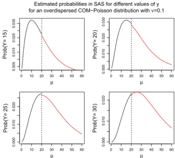
functions to compute the probability mass by simply trun-cating the normalisation constant up to a specified precision. The latter package offers the ability to compute the associ-ated COM-Poisson regression coefficients (in a maximum likelihood setting) only when the dispersion parameterν is independent of the covariates. TheCOUNTREGprocedure of the SAS/ETS (SAS Institute Inc 2014) software supports the COM-Poisson regression model (3), along with its orig-inal formulation bySellers and Shmueli(2010). In order to deal with the problem of evaluating the normalisation con-stantZ(μ, ν), the asymptotic approximation ofMinka et al. (2003) is used for μ > 20, while the normalisation con-stant is computed using truncation forμ ≤ 20 (when it is computationally easier). In this case, when one plots the probabilities ofY = y across different values ofμ (keep-ing the dispersion parameterνconstant), there exists a jump atμ =20. Figure1shows this discontinuity of the proba-bilities for an overdispersed COM-Poisson distribution with

ν = 0.1. The black line in each panel refers to the proba-bility when computing the normalisation constant, while the red line refers to the probability when using the asymptotic approximation.

3 Bayesian methods for COM-Poisson regression

models

The normalisation constant Z(μ, ν) in the COM-Poisson distribution is not available in closed form, hence evaluat-ing the likelihood can be computationally expensive. This makes it difficult to sample from the posterior distribution of the parameters in a COM-Poisson regression model. One possible solution is to use an asymptotic approximation of

Z(μ, ν) (Minka et al. 2003), which is known to be

rea-sonably accurate when μ > 10. Alternatively one could compute Z(μ, ν) by truncating its series at the kth term, but in order to achieve reasonable accuracy k may need to be very large. Evaluation of Z(μ, ν) could be avoided altogether using approximate Bayesian computation (ABC) methods. However, the resulting algorithms may not sam-ple from the distribution of interest and are usually much

0 10 20 30 40 50 60 0.005 0.015 0.025 0.035 μ Prob(Y= 15 ) 0 10 20 30 40 50 60 0.000 0.010 0.020 0.030 μ Prob(Y= 20 ) 0 10 20 30 40 50 60 0.000 0.010 0.020 μ Prob(Y= 25 ) 0 10 20 30 40 50 60 0.000 0.010 0.020 μ Prob(Y= 30 )

Estimated probabilities in SAS for different values of y for an overdispersed COM−Poisson distribution with ν=0.1

Fig. 1 Probabilities computed in SAS for different values ofμ. The

blackandred linesrefer to the probabilities when computing the

nor-malisation constant and when its asymptotic approximation is used. (Color figure online)

less efficient than standard MCMC algorithms which assume that the normalisation constants are known or cheap to com-pute. We overcome the problem of having an intractable likelihood by means of an MCMC algorithm that takes advantage of the exchange algorithm and the sampling tech-nique of Sect. 3.1. This algorithm is almost as efficient as one assuming the normalisation constants are readily avail-able.

3.1 Rejection sampling from the COM-Poisson distribution

This section sets out a simple, yet efficient method for sam-pling from the COM-Poisson distribution without having to evaluate its normalisation constant. This method will be a key part of the exchange algorithm proposed in Sect.3.4.

Suppose we want to generate a random variableY from the COM-Poisson distribution with probability mass func-tion p(y|θ) = q_Zθ₍(_θy₎) where θ = (μ, ν),q_θ(y) =

μy

y!

_ν and Z(θ) = _yq_θ(y). Denote by m the mode of the COM-Poisson distribution, i.e., m = μ and denote by s= √μ/√νits approximate standard deviation.

We construct an upper bound for the COM-Poisson distri-bution based on a piecewise geometric distridistri-bution. We start by defining three cut-off points,m−s,m,m+s. For the sake of simplicity, we assume thatm−s≥0; otherwise, we can simply omit the part of the upper bound falling to the left of 0.

Now consider a distribution with p.m.f. proportional to r_θ(y)= ⎧ ⎪ ⎪ ⎪ ⎪ ⎪ ⎪ ⎪ ⎪ ⎪ ⎨ ⎪ ⎪ ⎪ ⎪ ⎪ ⎪ ⎪ ⎪ ⎪ ⎩ q_θ(m−s)·m−s μ ν·(m−s−y) fory=0, . . . ,m−s qθ(m−1)· m−1 μ _ν·(m−1−y) fory=m−s+1, . . . ,m−1 q_θ(m)· μ m+1 _ν·(y−m) fory=m, . . . ,m+s−1 q_θ(m+s)·m+μs+1 ν·(y−m−s) fory=m+s,m+s+1, . . . (4) By constructionr_θ(y)≥q_θ(y).

For instance, ify∈ {m+1, . . . ,m+s−1}, then

q_θ(y)1/ν = μ y y! = μm m! =q_θ(m)1/ν y x₌m₊1 μ x ≤mμ+1 ≤q_θ(m)1/ν _μ m+1 y−m =r_θ(y)1/ν. (5)

In contrast to the COM-Poisson distribution, the piece-wise geometric distribution has a closed-form normalisation constant, Zg(θ)= ∞ y=0 r_θ(y)=q_θ(m−s) 1− m−s μ ₍m−s+1)ν 1− m−s μ ν +q_θ(m−1) 1− m−1 μ ₍s−1)ν 1− m−1 μ _ν +q_θ(m) 1− μ m+1 sν 1− μ m+1 _ν +q_θ(m+s) 1 1− μ m+s+1 _ν. (6) ClearlyZ(θ)≤ Zg(θ). Then, lettingg_θ(y)=P_θ(Y =y)=

r_θ(y)

Zg(θ) be the normalised p.m.f. corresponding torθ(y), one has that p(y|θ)= qθ(y) Z(θ) ≤ r_θ(y) Z(θ) = Zg(θ) Z(θ) r_θ(y) Zg(θ) = Zg(θ) Z(θ)gθ(y). This suggests sampling from p(y|θ) using the rejection method, with Z_Zg₍(_θθ₎)g_θ(y)as rejection envelope: a candidate yis drawn fromg_θ(y)and accepted with probability

p(y|θ) Zg(θ) Z(θ)gθ(y) = q_θ(y) Z(θ) Zg(θ) Z(θ) r_θ(y₎ Zg(θ) =qθ(y) r_θ(y), which only involves unnormalised densities.

We can sample fromg_θ(y)using a simple two-stage sam-pling procedure. First decide which part of the piecewise

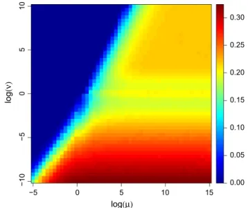
−5 0 5 10 15 −10 − 5 05 1 0 log(μ) log (ν) 0.00 0.05 0.10 0.15 0.20 0.25 0.30

Fig. 2 Rejection rate of the rejection sampler for the COM-Poisson distribution as a function of log(μ)and log(ν). The rejection rates were estimated based on samples of size 106

geometric distribution to sample from, according to proba-bilities proportional to the terms in (6). Then sample from the selected truncated geometric distribution using the inverse c.d.f. method, which is very efficient as the inverse c.d.f. is known in closed form.

The instrumental distribution in (4) is based on the same principle as the upper bounds used in the retrospective sam-pling algorithm proposed by Chanialidis et al. (2014). In contrast to the arbitrarily precise upper bound required for the retrospective algorithm, the bounds set out above are based on a trade-off between achieving a high acceptance rate while at the same time keeping the instrumental distribution simple so that sampling from it is computationally efficient. Figure2 shows the rejection rate of the above sampling algorithm as a function of the two parametersμandν. For most values ofμandν, the rejection rate is less than 30% and one can draw 106realisations from the COM-Poisson distribution in one second on a modern desktop computer (Intel Core i5).

Using a tighter rejection envelope (say by using more than four geometric pieces) yields a small reduction in the rejec-tion rate, but overall the computarejec-tional cost increases.

Finally, our proposed rejection algorithm in close in spirit to the basic adaptive rejection sampling technique (Gilks and Wild 1992) that constructs piecewise exponential proposal distributions which are adaptively refined using previously rejected samples.

3.2 Exchange algorithm

Møller et al.(2006) presented a Metropolis-Hastings algo-rithm for cases where the likelihood function involves an intractable normalisation constant that is a function of the

parameters. The idea behind this algorithm is to enlarge the state of the Markov chain to include, beside the parameterθ, an auxiliary variabley∗defined on the same sample space as the data y = (y1, . . . ,yn). Suitable choice of the proposal

distribution ensures that the Metropolis-Hastings acceptance ratio is free of normalisation constants.Murray et al.(2006) proposed a modification, known as the exchange algorithm, which still generates at each step y∗, but only updates the parameterθ if the move is accepted. To describe this algo-rithm, let us suppose that the sampling model p(y|θ)can be written as p(y|θ) = q_Zθ₍(_θy₎) where q_θ(y)is the unnor-malised probability density and the normalisation constant Z(θ)= _yq_θ(y)or Z(θ)= q_θ(y)dyis unknown. This can easily be extended to the case where theyi are not i.i.d.

(i.e., instead of p(y|θ)andq_θ(y)we will have pi(y|θ)and

qi,θ(y)since the sampling model and its unnormalised

prob-ability density will be different for each observation). For each MCMC update, first a candidate parameterθ∗is generated from the proposal distributionh(θ∗|θ); then aux-iliary datay∗are drawn from the sampling modelp(y∗|θ∗), conditional on the candidate parameter value. The candidate θ∗_{is accepted with probability min{1,a}. The computation}

of the acceptance ratioais detailed below, where we contrast it with the acceptance ratio in a standard Metropolis-Hastings algorithm; in both we assume that the proposal density is symmetric in its two arguments, i.e.,h(θ|θ∗)=h(θ∗|θ). In the exchange algorithm we have:

a= p(y|θ ∗_)p(θ∗_)p(y∗_|θ)h(θ|θ∗₎ p(y|θ)p(θ)p(y∗|θ∗)h(θ∗|θ), = i q_θ∗(yi) Z(θ∗) p(θ∗)h(θ|θ∗)_i qθ(y∗i) Z(θ) i q_θ(yi) Z(θ) p(θ)h(θ∗|θ)i q_θ∗(y_i∗) Z_(θ∗₎ , = iqθ∗(yi) p(θ∗)_iq_θ(y_i∗) iqθ(yi) p(θ)iqθ∗(yi∗) , (7)

while in the Metropolis-Hastings algorithm:

a= p(y|θ ∗_)p(θ∗_)h(θ|θ∗₎ p(y|θ)p(θ)h(θ∗|θ) , = i q_θ∗(yi) Z(θ∗) p(θ∗)h(θ|θ∗) i q_θ(yi) Z_(θ) p(θ)h(θ∗|θ) , = i q_θ∗(yi) Z(θ∗) p(θ∗) i q_θ(yi) Z(θ) p(θ) . (8)

Notice how the acceptance ratioafor the standard Metropo-lis-Hastings algorithm involves the ratio of normalisation constants _ZZ₍(_θθ∗)₎, which makes its computation hard. In the expression for the exchange algorithm, the ratio _ZZ₍(_θθ∗)₎

can-cels out and it is replaced by qθ(y∗i)

q_θ∗(y_i∗), suggesting that the latter

can be thought of as an importance sampling estimate for the former. We refer toMurray et al.(2006) for further discussion of the exchange algorithm.

Recently, Lyne et al. (2015) provided the first practi-cal and asymptotipracti-cally correct MCMC method for doubly intractable distributions that does not require exact sam-pling. This was done by constructing unbiased estimates of the reciprocal normalisation constant 1/Z(θ)using unbiased estimates of Z(θ) obtained by importance sampling. The pseudo-marginal approach byAndrieu and Roberts(2009) is then adapted to use these estimates to form an MCMC algo-rithm. Finally,Wei and Murray (2016) construct unbiased estimates of reciprocal normalisation constants by applying Russian roulette truncations to a Markov chain rather than an importance sampler. However, given that we can draw exact samples from the COM-Poisson distribution at very little computational cost there is no need to resort to these methods.

We discuss next the prior distributions for the regression coefficientsβ andδin the COM-Poisson regression model in (3).

3.3 Choice of prior for the regression coefficients For the priors of the regression coefficients, one can choose between a plethora of distributions. For the rest of the paper we will focus on three Bayesian COM-Poisson regression models; each one with a vague multivariate normal prior on β and a different prior for δ. The first model uses vague multivariate normal priors for both the regression coefficients β andδwith mean zero and a variance of 106, while the other two models use a shrinkage prior (lasso or spike and slab) forδ. The motivation behind using a penalty for large values of the regression coefficients of the variance is not just variable selection. Putting a penalty on the coefficients is a way of having the Poisson regression model as the “baseline” model. The aforementioned models can be specified as:

Lasso prior δ|t2j ∼Np(0,Dt) t2_j|λ2∼Exp(λ 2 2 ) λ2_∼ Gamma(a,b) Dt =diag(t12, . . . ,t 2 p)

Spike and slab prior δ|t2_j, φj∼Np(0,Dt)

t2_j ∼IG(a,b)

φj|ω∼(1−ω)I0()+ωI1()

ω∼U(0,1)

Dt=diag(t12φ1, . . . ,t2pφp)

where the first column represents a model with a lasso prior, while the second column represents a model with a spike and slab prior. The first model uses a conditional (on the variance) Laplace prior for the regression coefficientsδand

takes advantage of the representation of the Laplace as a scale mixture of normals with an exponential mixing density (Park and Casella 2008). Themaximum a posteriori(MAP) solu-tion, under the aforementioned Laplace prior, is identical to the estimate for the standard (non-Bayesian) lasso proce-dure. The idea behind the second model is that the prior of every regression coefficient is a mixture of a point mass at zero and a diffuse uniform distribution elsewhere. This form of prior is known as a spike and slab prior (Mitchell and Beauchamp 1988). The parameterωcontrols how likely each of the binary variablesφj is to equal 1. Since it

con-trols the size of the models, it can be seen as a complexity parameter.

3.4 MCMC sampling

For the COM-Poisson regression model, the acceptance ratio in (7) for the exchange algorithm becomes

a= iqθ∗(yi) p(β∗)p(δ∗)_iq_θ(y_i∗) iqθ(yi) p(β)p(δ)_iq_θ∗(y_i∗) , (9)

whereθ =(β,δ). In the sampler, we make use of two dif-ferent kinds of moves, in order to reduce the correlation between successive samples of the regression coefficientsβ andδ. Each sweep of the MCMC sampler performs these two moves in a sequence. The first proposes a move fromβto β∗_{and afterwards fromδtoδ}∗_{. The second proposes a move}

from (βi, δi) to (βi∗, δi∗) fori =1,2, . . . ,p, where pis the

number of variables. The first move is meant to address pos-terior correlation between coefficients of different covariates. The second move is meant to address posterior correlation between coefficients for the mean and coefficients for the dispersion.

The two kinds of moves of the MCMC algorithm can be specified as

A. First kind:

1. We drawβ∗ ∼ h(·|β) where the proposalh()is a multivariate Gaussian centred atβ. Specifically, Current value θi =(μi, νi), μi =exp{x_iβ}, νi =exp{−x_iδ}, Proposal θi∗=(μ∗i, νi∗), μ∗ i =exp{xiβ∗}, ν∗ i =νi, (10) where for the unnormalised COM-Poisson densities in (9) we have, q_θi(yi)= μyi i yi! _νi , q_θ∗ i(yi)= _(μ∗ i) yi yi! _ν∗ i , q_θi(y_i∗)= ⎛ ⎝μ y_i∗ i y_i∗! ⎞ ⎠ νi , q_θ∗ i(y ∗ i)= (μ∗ i) y_i∗ y∗_i! _ν∗ i . (11) 2. We now drawδ∗∼h(·|δ)where the proposalh()is a

multivariate Gaussian centred atδ. Specifically, Current value θi =(μi, νi), μi =exp{x_iβ}, νi =exp{−x_iδ}, Proposal θ∗ i =(μi∗, νi∗), μ∗ i =μi, νi∗=exp{−xiδ∗} (12) where the unnormalised COM-Poisson densities can be evaluated as in (11).

B. Second kind: For j=1, . . . ,p:

We drawβ∗_j ∼h(·|βj)andδ∗j ∼h(·|δj)where the

proposal distributionh()is a univariate Gaussian cen-tred atβj, δjrespectively and forl= jcopyβ_l∗=βl

andδ∗_l =δl. Specifically, Current value θi =(μi, νi), μi =exp{xiβ}, νi =exp{−xiδ}, Proposal θ∗i =(μ∗i, νi∗), μ∗i =exp{xi β∗}, νi∗=exp{−xiδ∗} (13) where the unnormalised COM-Poisson densities can be evaluated as in (11).

Each sweep of the MCMC algorithm performs both afore-mentioned moves i.e., we first update (βi, δi) for i =

1, . . . ,pand then updateβandδseparately; there arep+2 accept/reject decisions within each iteration of the MCMC algorithm.

In order to assess the computational efficiency of the proposed MCMC sampler, we have compared the effective sample size (ESS) per second of the proposed method to the one of a vanilla MCMC sampler for Poisson regression. We have simulated Poisson-distributed data (i.e.,ν=1), for which the latter sampler has used the closed-form expression of the normalisation constant. The ESS per second in the lat-ter case is only 10 times higher than the one for our proposed MCMC sampler, i.e., in order to get the same effective sample size the proposed method takes about 10 times as long. This factor of about 10 can be broken down into a factor of about 2 caused by the slower mixing of the exchange algorithm and a factor of about 5 caused by the higher computational cost of evaluating the acceptance ratio.

4 Simulation and case studies

4.1 Simulation

As already mentioned, the COM-Poisson regression model is a flexible alternative to count data models typically used in the literature, such as Poisson or negative binomial regres-sion. The key strength of the COM-Poisson regression model is its ability to differentiate between a covariate’s effect on the mean of the response variable and its effect on the (excess) variance. This can be seen if we simulate from the overdis-persed Poisson regression model (3), with

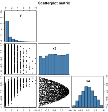
xi =(1,xi1,xi2,xi3,xi4), β=(0,0,0,0.3,2), ηi =xi β, Yi ∼Poi(exp(ηi)), (14) where xi j ii d ∼ U(−1,1), j = 1,2,3 and xi4|xi3 ∼ U(−ai,ai)withai = 1−xi3 2 (fori = 1,2, . . . ,n, where nis the number of observations). In this setup the range, and thus the dispersion, ofxi4 depends on xi3. The larger xi3, the smaller the dispersion ofxi4. However, xi3andxi4are uncorrelated.

An overdispersed regression model is then obtained by omittingxi4from the model specification, which corresponds toxi4not being directly observable. Becausexi3is related to the dispersion ofxi4, the degree of overdispersion ofYi

depends onxi3as well. In this case, the third covariate has a positive effect on the mean of the response variable (i.e., the value of the regression coefficient is positive) and a negative effect on its variance since higher values ofxi3will result in smaller dispersion for the covariatexi4. Thus, the dispersion of the response variable will also be smaller. Figure3shows the relationship between the response variables and the two covariatesxi3andxi4.

Our intention behind this simulation is not model selec-tion; our aim is to show that the parameter estimates from both the Poisson and negative binomial models may be dis-torted due to the effects of some covariates on the variance of the response variable.

We simulaten=1000 observations, which have empiri-cal mean and variance of 1.36 and 2.37, respectively. The 95 and 68% credible intervals for the coefficients for the Pois-son, negative binomial, and COM-Poisson regression model can be seen in Figs.4 and5. Figure 4 shows the credible intervals for the regression coefficients ofμfor all the mod-els.

The results for the Poisson and negative binomial mod-els both lead to the conclusion that the third covariate has a negative effect on the mean of the response variable. This happens due to the covariate having a negative effect on the variance of the response variable. On the other hand, the COM-Poisson regression model correctly identifies all

0 2 4 6 8 10 02468 1 0 y −1.0 −0.5 0.0 0 .5 1.0 x3 0 2 4 6 8 10 −1.0 −0.5 0.0 0 .5 1.0 −1.0 −0.5 0.0 0.5 1.0 −1.0 −0.5 0.0 0.5 1.0 −1.0 −0.5 0.0 0 .5 1.0 x4 Scatterplot matrix

Fig. 3 Scatterplot matrix which focuses on the relationship between the response variables and the covariatesxi3andxi4

−1.5 −1.0 −0.5 0.0 0.5 1.0 1.5 var3 var2 var1 intercept Poisson Neg. binomial COM−Poisson Regression coefficients for μ

Fig. 4 Simulation: 95 and 68% credible intervals for the regression coefficients ofμ. The latter are plotted with a shorter andthicker line

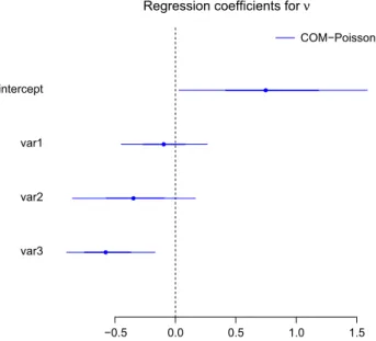
regression coefficients for the mean of the response variable. The credible intervals for the regression coefficients ofνfor the COM-Poisson model can be seen in Fig.5. The only pos-terior credible interval that does not include zero is the one for the third covariate (the one for the intercept is also wholly positive, although the lower end is very close to 0).

In order to generalise the results of the previous simula-tion, we have simulated 100 different samples from the model in (14) each one comprised ofn =1000 observations. The

−0.5 0.0 0.5 1.0 1.5 var3 var2 var1 intercept COM−Poisson Regression coefficients for ν

Fig. 5 Simulation: 95 and 68% credible intervals for the regression coefficients ofν. The latter are plotted with a shorter andthicker line Table 1 Number of times, out of 100 different replications of the model in (14), that the 95% credible interval for the coefficient of the third covariate is wholly negative, includes 0, or is wholly positive

Negative Includes 0 Positive

Poisson 6 88 6

Negative binomial 1 94 5

COM-Poisson 0 20 80

results can be seen in Table1. The Poisson and negative binomial models conclude that there is a positive effect of the third covariate on the response variable, in only 6 and 5 samples respectively. The COM-Poisson, on the other hand, infers a positive effect of the third covariate in 80 samples. 4.2 Publications by Ph.D. students

Long(1990) examined the effect of education, marriage, fam-ily, and the mentor on gender differences in the number of published papers during the Ph.D. studies of 915 individ-uals. The population was defined as all male biochemists who received their Ph.D.’s during the periods 1956–1958 and 1961–1963 and all female biochemists who obtained their Ph.D.’s during the period 1950–1967. Some of the vari-ables that were used in the paper are shown in Table2. For ease of interpretation, we standardise all non-binary covari-ates by subtracting their mean and dividing by their standard deviation.

The study found, amongst other things, that females and Ph.D. students having children publish fewer (on average) papers during their Ph.D. studies. In addition, having a men-tor with a large number of publications in the last three years

Table 2 Description of variables

Variable Description

Gender of student Equals 1 if the student is female; else 0

Married at Ph.D. Equals 1 if the student was married by the year of the Ph.D.; else 0 Children under 6 years old Number of children less than 6

years old at the year of the students Ph.D.

Ph.D. prestige Prestige of the Ph.D. program in biochemistry based on studies. Unranked institutions were assigned a score of 0.75, while ranked institutions had scores ranging from 1 to 5

Mentor Number of articles produced by Ph.D. mentor during the last 3 years

has a positive effect on the number of publications of the Ph.D. student. We will focus on the students with at least one publication (640 individuals) with empirical mean and variance of 1.42 and 3.54, respectively, a sign of overdisper-sion. Note that after focusing on the students with at least one publication, we subtract 1 from each student’s number of publications (e.g. the 246 students that had 1 publication in the original dataset are represented with a 0 in the final dataset). Removing the students with no publications (275 students out of the 915 students in the original dataset) allows us to fit a simple parametric model on the subset instead of a more complex alternative on the original dataset (e.g. zero-inflated model, hurdle model, non-parametric model). Thus, we only compare the Poisson, negative binomial, and the COM-Poisson regression models.

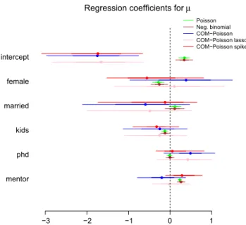
Figure6shows the 95 and 68% credible intervals for the regression coefficients ofμfor all the regression models. The Poisson and negative binomial models have similar results. The only difference between them is that for the latter model the 95% posterior interval on the effect of having children includes zero. The gender of a Ph.D. student and the number of articles by the Ph.D. mentor are the only covariates that have credible intervals that do not include zero, for both the Poisson and negative binomial models.

Specifically, these models conclude that female Ph.D. stu-dents publish less on average than male Ph.D. stustu-dents and that a mentor who has published a lot of articles has a positive effect on the number of articles of the Ph.D. student. On the other hand for the COM-Poisson models, the previous two covariates seem to not have an effect on the mean of the num-ber of articles published by a Ph.D. student. It must be noted that there are four male Ph.D. students with a large number of articles published (11,11,15,18) that could be considered as outliers. If these four students are taken out of the data

−3 −2 −1 0 1 mentor phd kids married female intercept

Regression coefficients for μ

Poisson Neg. binomial COM−Poisson COM−Poisson lasso COM−Poisson spike

Fig. 6 Publication data: 95 and 68% credible intervals for the regres-sion coefficients ofμ. The latter are plotted with a shorter andthicker line −1.0 −0.5 0.0 0.5 1.0 1.5 2.0 mentor phd kids married female intercept COM−Poisson COM−Poisson lasso COM−Poisson spike Regression coefficients for ν

Fig. 7 Publication data: 95 and 68% credible intervals for the regres-sion coefficients ofν. The latter are plotted with a shorter andthicker line

set, the gender covariate does not have a significant effect for the Poisson and negative binomial models. In addition, the empirical means of the male and female Ph.D. students are 1.5 and 1.2, respectively, while the empirical median is 1 for both genders. Thus the COM-Poisson regression model seems to be doing a better job at not concluding that there is an effect of the gender covariate.

Figure7shows the 95 and 68% credible intervals for the regression coefficients ofνfor the COM-Poisson regression models. This figure shows that there seems to be a positive

effect of the “mentor” covariate on the variance of the articles of the Ph.D. student. The more articles a mentor publishes (during the last 3 years) the larger the variance for the number of articles published by a Ph.D. student. This seems to be reinforced further when we look at the empirical variance of students having mentors with an above average number of articles published versus students having mentors with less than average number of articles published. The empirical variance for the former group is 5.8, with the latter group having a variance of 2.1, respectively (ratio of around 2.8). The corresponding empirical means are 1.9 and 1.2 (ratio of around 1.6). In Poisson-distributed data, one would expect the ratios to be roughly equal.

4.3 Fertility data

This section uses data fromWinkelmann(1995) on the num-ber of births given by a cohort of women in Germany. The data consist of 1243 women over 44 in 1985. The explanatory variables that were used can be seen in Table3.

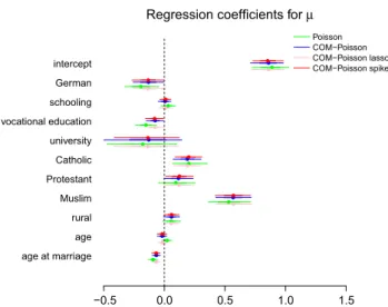
The empirical mean and variance of the response are 2.39 and 2.33, respectively. The unconditional variance is already slightly smaller than the unconditional mean. Includ-ing covariates the conditional variance will reduce further, thus suggesting that the data show underdispersion. For this reason, the negative binomial model was not used in this con-text. The results can be seen in Figs.8 and9. The credible intervals for the coefficients ofμ are similar across all the models. Looking at Fig.9we can see the credible intervals for the coefficients ofν. The posterior intervals that do not include zero refer to the vocational education, age, and age at marriage.

Table 3 Description of variables

Variable Description

Nationality Equals 1 if the woman is German; else 0

General education Measured as years of schooling Post-secondary education

(vocational training)

Equals 1 if the woman had vocational training; else 0 Post-secondary education

(university)

Equals 1 if the woman had a university degree; else 0

Religion The woman’s religious

denomination (Catholic, Protestant, Muslim) with other or none as the baseline group Area of residence Equals 1 if its a rural area; else 0

Age Age of the woman at the time of

the survey

Age at marriage Age of the woman at the time of marriage

−0.5 0.0 0.5 1.0 1.5 age at marriage age rural Muslim Protestant Catholic university vocational education schooling German intercept Poisson COM−Poisson COM−Poisson lasso COM−Poisson spike

Regression coefficients for μ

Fig. 8 Fertility data: 95 and 68% credible intervals for the regression coefficients ofμ. The latter are plotted with a shorter andthicker line

−0.5 0.0 0.5 1.0 1.5 age at marriage age rural Muslim Protestant Catholic university vocational education schooling German intercept COM−Poisson COM−Poisson lasso COM−Poisson spike Regression coefficients for ν

Fig. 9 Fertility data: 95 and 68% credible intervals for the regression coefficients ofν. The latter are plotted with a shorter andthicker line

For model selection, we will use the deviance information criterion (DIC) bySpiegelhalter et al. (2002). This can be seen as a Bayesian alternative model selection tool to AIC and BIC. A smaller DIC indicates a better fit to the data set. The results for both data sets (published papers and fertility data) can be found in Table4and show that the COM-Poisson models outperform the Poisson and the negative binomial models in both examples.

5 Comparing MCMC algorithms for

COM-Poisson regression models

Besides showing the flexibility the COM-Poisson distribu-tion offers, the goal of this paper is to propose an MCMC algorithm for COM-Poisson regression models more

effi-Table 4 Deviance information criterion for all models and all data sets with the minimum DIC in bold

Ph.D. data Fertility data

Poisson 2251.09 4214.55

Negative binomial 2108.05 –

COM-Poisson 2056.77 4121.92

COM-Poisson (lasso) 2058.05 4121.43

COM-Poisson (spike and slab) 2062.23 4121.74

−3 −2 −1 0 1 mentor phd kids married female intercept COM−Poisson (exchange) COM−Poisson (bounds)

Regression coefficients for μ

Fig. 10 Publication data: 95 and 68% credible intervals for the regres-sion coefficients ofμ. The latter are plotted with a shorter andthicker line

cient than the exact MCMC algorithm ofChanialidis et al. (2014). The main idea behind the algorithm given in Cha-nialidis et al. (2014) is to take advantage of a sequence of increasingly and arbitrarily precise lower and upper bounds on the likelihood, resulting in bounds on the target density and the acceptance probability of the Metropolis-Hastings algorithm. This sequence of arbitrarily precise bounds is cre-ated by increasing the number of terms that are computed exactly for the estimation of the normalisation constant and using piecewise geometric bounds for the remaining terms. Assuming that πˇn andπˆn are the lower and upper bounds

of the target density afternrefinements, the proposed algo-rithm for deciding on the acceptance ofθ∗then proceeds as follows:

1. DrawU∼Unif(0,1)and set the number of refinements n=0.

2. Computeπˇnandπˆnand compare them toU.

– IfU≤ ˇπn,accept the candidate value.

– IfU>πˆn,reject the candidate value.

– Ifπˇn < U < πˆn,refine the bounds, i.e increasen

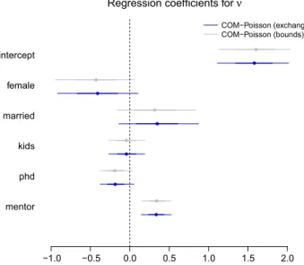
−1.0 −0.5 0.0 0.5 1.0 1.5 2.0 mentor phd kids married female intercept COM−Poisson (exchange) COM−Poisson (bounds)

Regression coefficients for _ν

Fig. 11 Publication data: 95 and 68% credible intervals for the regres-sion coefficients ofν. The latter are plotted with a shorter andthicker line

Traceplot for regression coefficients of μ for the exchange algorithm

0 10000 20000 30000 40000 50000 60000 −4 −3 −2 −1 0 intercept 0 10000 20000 30000 40000 50000 60000 −3 −2 −1 0 1 2 female 0 10000 20000 30000 40000 50000 60000 −4 −3 −2 −1 0 1 married 0 10000 20000 30000 40000 50000 60000 −2.0 −1.0 0.0 0 .5 1.0 kids 0 10000 20000 30000 40000 50000 60000 −1.0 0.0 0 .5 1.0 1 .5 phd 0 10000 20000 30000 40000 50000 60000 −1.5 −0.5 0.0 0 .5 mentor

Fig. 12 Publication data: Traceplots for the regression coefficients of

μfor the exchange algorithm

We will now compare the algorithm presented in Chania-lidis et al.(2014) with the MCMC algorithm presented in this paper, using the publications data discussed in Sect.4.2. Both MCMC algorithms include the two kinds of moves pre-sented in Sect.3.4, have a burn-in period of 20,000 iterations and a posterior sample size of 60,000.

Figures10and11show the 95 and 68% credible intervals for the regression coefficients ofμandνfor both MCMC algorithms. It can be seen that the “exchange” MCMC gives similar results as the “bounds” MCMC.

Traceplot for regression coefficients of μ for the bounds algorithm

0 10000 20000 30000 40000 50000 60000 −4 −3 −2 −1 0 intercept 0 10000 20000 30000 40000 50000 60000 −3 −2 −1 0 1 2 3 female 0 10000 20000 30000 40000 50000 60000 −4 −3 −2 −1 0 1 married 0 10000 20000 30000 40000 50000 60000 −2 −1 0 1 kids 0 10000 20000 30000 40000 50000 60000 −1.0 0.0 0 .5 1.0 1.5 2.0 phd 0 10000 20000 30000 40000 50000 60000 −1.5 −0.5 0.0 0 .5 1.0 mentor

Fig. 13 Publication data: Traceplots for the regression coefficients of

μfor the bounds algorithm

Traceplot for regression coefficients of ν for the exchange algorithm

0 10000 20000 30000 40000 50000 60000 1.0 1 .5 2.0 intercept 0 10000 20000 30000 40000 50000 60000 −1.0 −0.5 0.0 0 .5 female 0 10000 20000 30000 40000 50000 60000 −0.5 0.0 0.5 1 .0 1.5 married 0 10000 20000 30000 40000 50000 60000 −0.4 −0.2 0.0 0.2 0.4 kids 0 10000 20000 30000 40000 50000 60000 −0.4 −0.2 0.0 0 .2 phd 0 10000 20000 30000 40000 50000 60000 0.0 0 .2 0.4 0.6 mentor

Fig. 14 Publication data: Traceplots for the regression coefficients of

νfor the exchange algorithm

Traceplots for the regression coefficients of μ can be seen in Figs.12,13, while the traceplots for the regression coefficients ofν can be seen in Figs.14,15. Both MCMC algorithms seem to mix well.

The main difference between the two algorithms is the computation time. For the “exchange” MCMC algorithm the computation time was 14 min, while the “bounds” MCMC

Traceplot for regression coefficients of ν for the bounds algorithm 0 10000 20000 30000 40000 50000 60000 1 .01 .5 2 .02 .5 intercept 0 10000 20000 30000 40000 50000 60000 −1.5 −1.0 −0.5 0.0 0 .5 female 0 10000 20000 30000 40000 50000 60000 −0.5 0.0 0 .5 1.0 1 .5 married 0 10000 20000 30000 40000 50000 60000 −0.4 −0.2 0.0 0 .2 0.4 kids 0 10000 20000 30000 40000 50000 60000 −0.4 −0.2 0.0 0 .2 phd 0 10000 20000 30000 40000 50000 60000 0.0 0 .2 0.4 0 .6 mentor

Fig. 15 Publication data: Traceplots for the regression coefficients of

νfor the bounds algorithm

algorithm needed 238 min for the same number of iterations, seventeen times longer. A similar difference on the compu-tation time is seen on the fertility data set.

Tables5and6show the effective sample sizes (ESS) per minute for the regression coefficients of μ and ν respec-tively. In both tables and across all the regression coefficients, the “exchange” MCMC outperforms the “bounds” MCMC algorithm. The average ESS per minute for the “exchange” MCMC is 123.01 while for the “bounds” MCMC is 11.94.

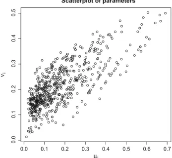
Figure16shows the scatterplot of the parametersμi,νi

fori = 1, . . . ,640. The parameters μi,νi were obtained

using the posterior sample of the “exchange” algorithm and substituting the posterior mean of each regression coefficient

βj, δjfor j =1, . . . ,6 in Eq. (3).

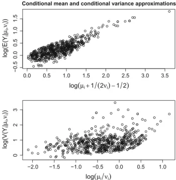
Figure 17 shows the conditional mean and variance approximations (on the log scale) seen at the start of Sect.2. Thex-axes refer to the right-hand side of the Eq. (2), while they-axes refer to the mean and variance of a COM-Poisson

0.0 0.1 0.2 0.3 0.4 0.5 0.6 0.7 0.0 0 .1 0.2 0 .3 0.4 0 .5 Scatterplot of parameters μi νi

Fig. 16 Publication data: Scatterplot of the parametersμandν distribution with parameters μi, νi. In order to compute

the mean and variance, we first estimated the probability mass function of the COM-Poisson distribution evaluation the normalisation constantZ(μi, νi)and then used the

defi-nitions of the mean and variance of a distribution. Figure18 shows a scatterplot of the conditional mean versus the con-ditional variance. The dotted line refers to the case where the conditional mean is equal to the conditional variance. In this case all the points are above the line, a sign of overdispersion.

Finally, we have used both MCMC algorithms on the publications and fertility data sets, with 5 different start-ing values and the “exchange” MCMC algorithm consis-tently outperforms the “bounds” MCMC. Due to constraints of space, we have only shown the results for one of those seeds on the smaller data set (i.e., publications data set).

R (R Core Team 2015) was used for all the computa-tions in this paper. Traceplots, density plots, autocorrelation plots (for every regression coefficient) and results for the Gel-man and Rubin diagnostic,Gelman and Rubin(1992), were Table 5 Effective sample size

per minute for the regression coefficients ofμ

β1 β2 β3 β4 β5 β6

“Exchange” MCMC 65.51 91.01 99.21 154.03 157.42 186.54 “Bounds” MCMC 6.32 8.40 10.04 15.08 14.22 15.94

Table 6 Effective sample size per minute for the regression coefficients ofν

δ1 δ2 δ3 δ4 δ5 δ6

“Exchange” MCMC 58.87 91.86 74.67 168.63 161.44 166.85 “Bounds” MCMC 5.80 8.74 8.07 16.85 15.55 16.68

0.0 0.5 1.0 1.5 2.0 2.5 3.0 3.5 −0.5 0.0 0.5 1 .0 1.5

Conditional mean and conditional variance approximations

log(μi+1 (2νi)−1 2) log (E( Yi | μi , νi )) −2.0 −1.5 −1.0 −0.5 0.0 0.5 1.0 0123 log(μi νi) log(V(Y i | μi , νi ))

Fig. 17 Publication data: Mean and variance approximations

0 1 2 3 4

02

468

1

0

Conditional mean vs conditional variance

E(Yi|μi,νi) V(Y i | μi , νi )

Fig. 18 Publication data: conditional mean versus conditional variance

employed to assess convergence of the MCMC samplers to the posterior distribution, using the coda package (Plummer et al. 2006). The plots for the credible intervals and the tra-ceplots of the regression coefficients were made using the mcmcplots package (Curtis 2015).

The code for both MCMC algorithms (“exchange” and “bounds”) is now available on Github.1

1_{https://github.com/cchanialidis/combayes}

6 Conclusions

In this paper, we presented a computationally more efficient MCMC algorithm for COM-Poisson regression compared to the alternative inChanialidis et al.(2014). We showed how rejection sampling, combined with the exchange algorithm, can be used to overcome the problem of an intractable likeli-hood in the COM-Poisson distribution. Finally, this allowed us to use a Bayesian COM-Poisson regression model and show its benefits, compared to the most common regression models for count data, through a simulation and two real-world data sets.

Open Access This article is distributed under the terms of the Creative Commons Attribution 4.0 International License (http://creativecomm ons.org/licenses/by/4.0/), which permits unrestricted use, distribution, and reproduction in any medium, provided you give appropriate credit to the original author(s) and the source, provide a link to the Creative Commons license, and indicate if changes were made.

References

Andrieu, C., Roberts, G.O.: The pseudo-marginal approach for efficient monte carlo computations. Ann. Stat.37, 697–725 (2009) Chanialidis, C., Evers, L., Neocleous, T., Nobile, A.: Retrospective

sam-pling in MCMC with an application to COM-poisson regression. Stat3(1), 273–290 (2014). doi:10.1002/sta4.61

Conway, R.W., Maxwell, W.L.: A queuing model with state dependent service rate. J. Ind. Eng.12, 132–136 (1962)

Curtis, S.M.: mcmcplots: Create plots from MCMC output. http:// CRAN.R-project.org/package=mcmcplots, r package version 0.4.2 (2015)

Dunn, J.: compoisson: Conway–Maxwell–Poisson Distribution.https:// CRAN.R-project.org/package=compoisson, r package version 0.3 (2012)

Gelman, A., Rubin, D.B.: Inference from iterative simulation using multiple sequences. Stat. Sci.7(4), 457–472 (1992)

Geyer, C.J.: Markov chain Monte Carlo maximum likelihood. In: Proceedings of Computing Science and Statistics: The 23rd Sym-posium on the Interface, Interface Foundation of North America, pp. 156–161 (1991)

Gilks, W.R., Wild, P.: Adaptive rejection sampling for Gibbs sampling. Appl. Stat.42, 337–348 (1992)

Guikema, S.D., Coffelt, J.P.: A flexible count data regression model for risk analysis. Risk Anal.28, 213–223 (2008). doi:10.1111/j. 1539-6924.2008.01014.x

Long, J.S.: The origins of sex differences science. Soc. Forces68(4), 1297–1315 (1990)

Lyne, A.M., Girolami, M., Atchadé, Y., Strathmann, H., Simpson, D.: On Russian roulette estimates for Bayesian inference with doubly-intractable likelihoods. Stat. Sci.30(4), 443–467 (2015). doi:10. 1214/15-STS523

Minka, T.P., Shmueli, G., Kadane, J.B., Borle, S., Boatwright, P.: Computing with the COM-poisson distribution. Tech. rep, CMU Statistics Department (2003)

Mitchell, T.J., Beauchamp, J.J.: Bayesian variable selection in linear regression. J. Am. Stat. Assoc.83(404), 1023–1032 (1988) Møller, J., Pettitt, A.N., Reeves, R., Berthelsen, K.K.: An

effi-cient Markov chain Monte Carlo method for distributions with intractable normalising constants. Biometrika 93(2), 451–458 (2006). doi:10.1093/biomet/93.2.451

Murray, I., Ghahramani, Z., MacKay, D.J.C.: MCMC for doubly-intractable distributions. In: Proceedings of the 22nd Annual Conference on Uncertainty in Artificial Intelligence (UAI-06), AUAI Press, pp. 359–366 (2006)

Park, T., Casella, G.: The Bayesian lasso. J. Am. Stat. Assoc.103(482), 681–686 (2008). doi:10.1198/016214508000000337

Plummer, M., Best, N., Cowles, K., Vines, K.: Coda: convergence diag-nostics and output analysis for MCMC. R News6(1), 7–11 (2006)

http://CRAN.R-project.org/doc/Rnews/

R Core Team: R: A language and environment for statistical comput-ing. R foundation for statistical computing, Vienna, Austria (2015)

http://www.R-project.org/

SASInstitute Inc (2014)SAS/ETS13.2 user’s guide. Cary, NC,http:// www.sas.com/

Sellers, K., Lotze, T.: COMPoissonReg: Conway–Maxwell–Poisson (COM-Poisson) regression. (2015)https://CRAN.R-project.org/ package=COMPoissonReg, r package version 0.3.5

Sellers, K.F., Shmueli, G.: A flexible regression model for count data. Ann. Appl. Stat.4(2), 943–961 (2010). doi:10.1214/09-aoas306

Shmueli, G., Minka, T.P., Kadane, J.B., Borle, S., Boatwright, P.: A useful distribution for fitting discrete data: revival of the Conway– Maxwell–Poisson distribution. J. R. Stat. Soc.: Ser. C54(1), 127– 142 (2005). doi:10.1111/j.1467-9876.2005.00474.x

Spiegelhalter, D.J., Best, N.G., Carlin, B.P., Van Der Linde, A.: Bayesian measures of model complexity and fit. J. R. Stat. Soc.: Ser. B64(4), 583–639 (2002). doi:10.1111/1467-9868.00353

Wei, C., Murray, I.: Markov chain truncation for doubly-intractable inference. (2016) ArXiv e-printsArXiv:1610.05672

Winkelmann, R.: Duration dependence and dispersion in count-data models. J. Bus. Econ. Stat.13(4), 467–474 (1995)