RCS Calculation Using Hybrid FDTD-NARX Technique

RCS Calculation Using Hybrid FDTD-NARX Technique

Nihar K. Sahoo*, Dhruba C. Panda, Rabindra K. Mishra, and Amit K. Sahu

Abstract—This paper amalgamates two uncorrelated techniques namely finite difference time domain technique (FDTD) and nonlinear autoregressive with exogenous input (NARX) neural network to achieve a faster computation of radar cross section (RCS). It generates only a limited number of FDTD data and uses them to train a NARX neural network. The data beyond this limited number for the FDTD come from the NARX prediction. Comparison of the performance of FDTD-NARX hybrid with other methods indicates good matching with better timing for RCS of electrically larger objects.

1. INTRODUCTION

RCS is an essential parameter in strategic applications [1]. It gives the electromagnetic signature of an object through radar technology. Therefore, it continues to be an essential subject of research. Its analytical expression is a complicated function of parameters like conductivity, permittivity, permeability, aspect angle, the shape of objects, and radar operating frequency. Its computation for a realistic object requires high computational resources. High-frequency asymptotic techniques like Geometrical Optics, Physical Optics [2], Geometrical Theory of Diffraction, Physical Theory of Diffraction, and Ray tracing methods [3–7] are the few examples for faster RCS computation. These methods are faster but problem dependent. The full-wave solvers like FDTD, MoM, and FEM are advantageous because of their adaptability to different geometric shapes [8]. However, for larger objects or high frequencies, they demand high computing resources and cost. Thus it is necessary to recast existing methods with techniques from other non-electromagnetic domains to reduce the high computing demand.

In this work, we consider time tested FDTD method [8–11] as the base for RCS calculation. Inherently, the computational resources for FDTD depend on the number of generated cells. Among the available techniques addressing these issues, different types of artificial neural networks (ANN) [12, 13] are prominent. Such methods, except NFDTD [14], are usually problem specific. With this consideration, the objective here is to limit the exponentially growing computational time and memory requirement that comes with increasing object size and frequency.

We know that for electromagnetic (EM) problems, FDTD is a time domain technique. The central part of FDTD is the time marching loop that generates scattered fields for each location in the problem domain. During implementation, an array at each location stores the time series field value. So, a time series predictor shall be useful in achieving the objective mentioned earlier. We propose to use NARX as the time series predictor in this paper. With a simple network structure [15], the NARX neural network is easy to implement, and it converges faster. Compared to other recurrent networks, it has limited feedback which comes only from the output neuron instead of hidden states. NARX network [15] is well suited for predicting the nonlinear system’s behaviour such as nonlinear active noise control, the design of nonlinear systems in the frequency domain [16], for power system load modelling, recursive identification for nonlinear ARX systems [17], etc.

Received 10 April 2019, Accepted 5 June 2019, Scheduled 22 June 2019 * Corresponding author: Nihar Kanta Sahoo ([email protected]).

2. NARX TIME SERIES PREDICTOR

NARX is a three-layer neural network with the nonlinear sigmoid transfer function in the hidden layer and a linear transfer function in the output layer. It has two inputs; one is exogenous input, and the other is feedback. This network contains embedded delays in both the inputs. They reduce the sensitivity of long-term dependencies and enhance learning capability [15]. The accuracy of prediction of the network depends on the number of hidden neurons and embedded memory elements. Thus, its output in functional form is

y(t) =f(y(t−1). . . y(t−do)x(t−1). . . x(t−di)) (1)

Here,f is a nonlinear function;di anddo are the input delay and output delay orders;x(t) andy(t) are

the input and output sequences, respectively at time t. Figure 1 shows the NARX network schematic. The output of the network is

y(t) = uo(t) (2)

uo(t) = Nh

h=1

(wohzh(t) +bo) (3)

zh(t) = f(uh(t)) (4)

uh(t) = di

i=0

wihx(t−i) + d0

j=0

wjhy(t−j) +bh (5)

In the above equation, uh(t) is the input to the hth hidden neuron, zh(t) the output of the hth hidden

neuron, uo(t) the network output, wih the weight from the ith exogenous input to hth hidden neuron,

wjhthe weight from thejthfeedback input tohthhidden neuron,wohthe weight fromhthhidden neuron

to the output, bh the hidden bias, bo the output bias, and Nh the number of hidden neurons. f is a

sigmoid transfer function at each hidden neuron. The network training uses known exogenous input and output time series to identify the nonlinear functional mapping. The performance measure of the training is mean square error (MSE). The lower the MSE is, the more accurate the prediction is. The expression for the MSE is

M SE= 1

n

n

i=1

(ˆyi−yi)2 (6)

where y_i and yi are the desired and network output values respectively for the ith sample, and n

is the number of data samples. The weight updation uses the Levenberg-Marquardt (LM) training algorithm [18, 19] resulting in

wk+1 = wk−Δwk (7)

Δwk =

JT(wk)J(wk) +μI

−1

JT (wk)e(wk) (8)

where wk denote the weight matrix at the kth iteration, I the identity matrix, μ the damping factor,

e(wk) the error vector of all the training samples, J the Jacobian matrix, andJT is its transpose. The

LM algorithm is an iterative technique. It finds the minimum of a function which is in the form of a sum of squares. It is like a combination of steepest descent and Gauss-Newton method. Its training follows two-way procedure; when the prediction is far from the target, the algorithm acts as a steepest descent method, and when the prediction is close to the target, it acts as a Gauss-Newton method. Its training time is low for less number of weights.

3. PROPOSED HYBRID MODEL

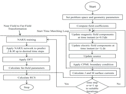
Figure 2 shows the block diagram of the proposed hybrid model. This model first uses the FDTD algorithm for a limited number of iterations to generate time series data for training of the NARX network. After training, the NARX predicts the time series data for future iterations. The time series data can be the fields or currents on a surface depending on the nature of the problem.

Figure 2. Block diagram of FDTD-NARX.

4. APPLICATION TO RCS (σ) CALCULATION

The analytical expression for RCS [9] of an object is

σ = 4πR2

_Es2

_Ei2

(9)

here,σ is the RCS;R is the range of the radar from the target;EiandEs are the scattered and incident

electric fields, respectively. It is a far-field parameter. Use of spherical coordinates is common in RCS calculation.

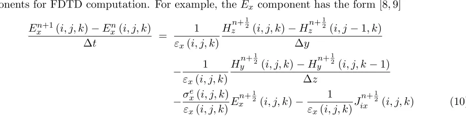
4.1. FDTD Formulation

components for FDTD computation. For example, theEx component has the form [8, 9]

E_xn+1(i, j, k)−E_xn(i, j, k)

Δt =

1

εx(i, j, k)

Hzn+12 (i, j, k)−Hn

+1₂

z (i, j−1, k)

Δy

− 1

εx(i, j, k)

Hn+12

y (i, j, k)−Hn

+1₂

y (i, j, k−1)

Δz

−σxe(i, j, k)

εx(i, j, k)E n+1₂

x (i, j, k)−

1

εx(i, j, k)J n+1₂

ix (i, j, k) (10)

After determination of the field components, the process described in [20] gives the far-field parameters

Lθ,Lϕ,Nθ,Nϕ, to find the RCS as given below

RCS_θ = k 2

8πη0Pinc|Lϕ

+η0Nθ|2 (11)

RCS_ϕ = k 2

8πη0Pinc|Lθ

+η0Nϕ|2 (12)

herePinc is the incident plane wave power.

Pinc=

1 2η0 |Einc

(ω)|2 (13)

5. IMPLEMENTATION

The FDTD formulation uses CPML boundary condition [21] and keeps the object under test (OUT) centred at the origin. A Gaussian plane wave illuminates the OUT. An imaginary cubic box encloses the OUT. The box is in the near field region of the OUT. On each of the six faces of the box

xp, xn, yp, yn, zp, zn, the surface equivalence theorem gives the surface currents (Js and Ms) from the

near scattered field values (E and H) obtained from FDTD formulation [20]. The equivalent currents of xp-face are

Js = ˆx×H = ˆx×(ˆxHx+ ˆyHy+ ˆzHz) = ˆzHy−yHˆ z (14)

Ms = −xˆ×E =−xˆ×(ˆxEx+ ˆyEy + ˆzEz) =−zEˆ y+ ˆyEz (15)

From Equations (14) and (15), four electric and magnetic scalar currents ofxp-plane areJy, Jz, My, Mz.

Here, Jy =−Hz, Jz =Hy, My =Ez, Mz =−Ey. A similar procedure gives all other surface currents.

Each of the six faces of the box shall have Nc×Nc cells. Each cell shall have two scalar electric and

magnetic currents. Thus, there is a storage requirement for a total of 4×6×N_c2 surface currents. Figure 3 illustrates the illumination of the FDTD domain for RCS calculation. Table 1 shows the parameters used in the FDTD code. The FDTD code runs for a limited number of iterations (N) depending on the OUT size, to generate training values of currents for the NARX. The plane wave

Table 1. FDTD coding parameters for OUT.

SN Parameters Sphere, Cube, Cylinder 1 Frequency of operation 100 MHz

2 Size of Cell λ/20

4 CPML boundary layer 6–8 cells 3 Source direction θ= 0◦, ϕ= 0◦ 5 Material parameters (r = 3, μr = 2)

Figure 3. Illustration of the FDTD domain for RCS calculation.

Table 2. NARX parameters.

Number of Hidden Neurons 20

Number of delays for both input 6

Training Algorithm Levenberg-Marquardt

source is exogenous input for NARX network. Table 2 shows the parameters used in the NARX neural network. In the NARX neural network, the initial weight values are randomly chosen between [−0.5,0.5]. The initial learning rate varies according to a standard procedure mostly remaining around 0.001. The trained NARX neural network predicts current values from (N+ 1) toNf (stable state) iterations. For

calculation of RCS in a single cut-plane the NARX needs to run (4×2×N_c2) times. Then the application of DFT gives the far-field parameters (Lθ, Lϕ, Nθ, Nϕ), completing the NF-FF transformation. After

that, Equations (11) and (12) give the RCS in the corresponding plane. Figure 4 shows a flow chart for implementation of the process.

6. RESULT DISCUSSION

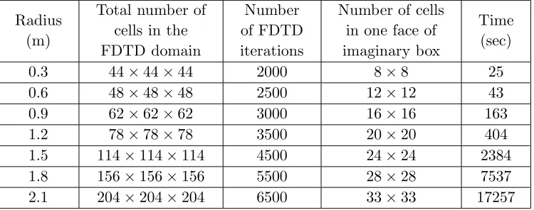
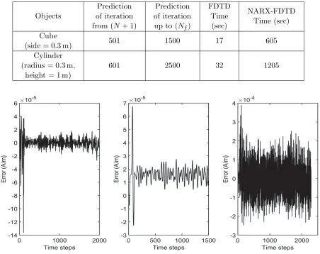
The coding and its execution uses a DELL PC with Intel Core i7 processor, 8 GB RAM, CN-ON4YC8-72200-63E-008V-A00 motherboard. Result validation uses commercial EM codes FEKO [22] and CST (time domain solver). Object samples include a cube of 0.3 m side length, a cylinder of 0.3 m radius, and 1 m height and seven spheres with radii varying from 0.3 m to 2.1 m in increments of 0.3 m. FEKO validation and comparison simulations use full-wave methods (FEM, MoM, FDTD) available in the package. The RCS calculations are at 100 MHz which is useful for long surveillance radar. Table 3 shows the number of cells for the FDTD domain and on one face of the imaginary box as well as the number of iterations with total computing time for different spheres. For the FDTD-NARX, Table 4 shows the prediction iteration numbers and the total computing time for different spheres. Exclusion of similar tables for other two objects is because the computing time depends on the size of the imaginary box, and irrespective of the shape of the OUT, its dimension shall determine the size of the imaginary box. However, Table 5 provides sample results for cube (side 0.3 m) and cylinder (radius 0.3 m and height 1 m) and compares performance time for standard FDTD and FDTD-NARX. Figure 5 shows the FDTD-NARX performance in terms of MSE stabilization considering a tolerance of better than 4 decimal places for sphere, cube, and cylinder, limiting the number of training epochs to 1000. The time step requirements are also available in Tables 3–5. Table 6 compares computing time of FDTD-NARX with other full-wave methods. Figures 6(a) and (b) respectively show the FDTD-NARX calculated RCS for the seven spheres in xz plane (ϕ = 0◦) and yz plane (ϕ= 90◦). Figure 6(c) shows a comparison of FDTD and NARX predicted surface current of a random point for the sphere (radius 0.3 m). For

Table 3. Computing time of FDTD for spheres of different radii.

Radius (m)

Total number of cells in the FDTD domain

Number of FDTD iterations

Number of cells in one face of imaginary box

Time (sec)

0.3 44×44×44 2000 8×8 25

0.6 48×48×48 2500 12×12 43

0.9 62×62×62 3000 16×16 163

1.2 78×78×78 3500 20×20 404

1.5 114×114×114 4500 24×24 2384

1.8 156×156×156 5500 28×28 7537

Table 4. Total computing time of the FDTD-NARX for spheres of different radii.

Radius (m) Prediction of iteration from (N + 1)

Prediction of iteration up to (Nf)

Time (sec)

0.3 701 2000 700

0.6 751 2500 1340

0.9 851 3000 2310

1.2 901 3500 3542

1.5 1001 4500 4998

1.8 1151 5500 7025

2.1 1251 6500 13588

Table 5. Total computing time of the FDTD-NARX for cube and cylinder of different size.

Objects

Prediction of iteration from (N + 1)

Prediction of iteration up to (Nf)

FDTD Time

(sec)

NARX-FDTD Time (sec)

Cube

(side = 0.3 m) 501 1500 17 605

Cylinder (radius = 0.3 m,

height = 1 m)

601 2500 32 1205

Figure 5. MSE performance of FDTD-NARX for different OUTs.

better understanding, Figures 7(a) and (b), respectively, show the FDTD-NARX calculated RCS for the sphere of radius 0.3 m in xz plane (ϕ = 0◦) and yz plane (ϕ = 90◦). Figures 8(a) and (b) and Figures 9(a) and (b) respectively show the FDTD-NARX calculated RCS for the cube and cylinder in

(a)

(b)

(c)

Figure 6. (a) Calculated RCS_θ of the spheres at 100 MHz in thexzplane. (b) Calculated RCS_ϕ of the spheres at 100 MHz in theyz plane. (c) A comparison of FDTD and NARX (predicted) surface current of a random point of sphere (radius 0.3 m).

Figures 7, 8, and 9 indicate that the OUTs are appreciably detectable in the rangeθ =−180◦ to −60◦ on thexzplane andθ= 0◦ to 180◦on theyzplane. In thexzplane, a blind point appears around

(a)

(b)

Figure 7. (a) Comparison of calculated RCS_θof the sphere at 100 MHz in thexzplane. (b) Comparison of calculated RCS_ϕ of the sphere at 100 MHz in theyz plane.

follow each other closely.

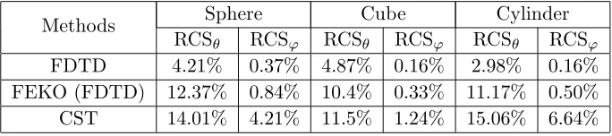
Comparisons of Tables 3, 4, and 5 indicate that for smaller objects, FDTD is efficient. However, as the object size increases, the FDTD-NARX technique catches up with the normal FDTD and outperforms it for a sphere with a radius larger than or equal to 1.8 m. Table 6 indicates that the FDTD-NARX outperforms other full-wave methods for the sphere of radius larger than 2.1 m. Table 7 compares the accuracy of the proposed method with other commercial codes and FDTD in terms of percentage of deviation. It is seen that the maximum percentage of deviation is 15%, and minimum percentage of deviation is 0.16%, which are easily tolerable. In this work, the spatial grid size in all

(b)

Figure 8. (a) Comparison of calculated RCS_θ of the cube at 100 MHz in thexzplane. (b) Comparison of calculated RCS_ϕ of the cube at 100 MHz in the yz plane.

(a)

(b)

Table 6. Computing time comparison of FDTD-NARX with other full-wave methods.

Methods Size (m) Computational time (sec)

FEM (FEKO, parallel computing) 2.1 15033

MoM (FEKO, parallel computing) 2.1 14266

FDTD (FEKO, parallel computing) 2.1 13698

FDTD 2.1 17257

FDTD-NARX 2.1 13588

Table 7. Percentage of deviation of proposed method with FDTD, FEKO (FDTD), and CST.

Methods Sphere Cube Cylinder

RCS_θ RCS_ϕ RCS_θ RCS_ϕ RCS_θ RCS_ϕ

FDTD 4.21% 0.37% 4.87% 0.16% 2.98% 0.16%

FEKO (FDTD) 12.37% 0.84% 10.4% 0.33% 11.17% 0.50% CST 14.01% 4.21% 11.5% 1.24% 15.06% 6.64%

cases isλ/20. In addition for FEKO, number of meshes is 137194 (tetrahedral) when using FEM and 346573 (tetrahedral) when using MoM.

7. CONCLUSION

The proposed integration of NARX with FDTD achieves the desired objective in RCS calculation of electrically large objects. For electrically small objects, standalone FDTD is a better choice. The NARX-FDTD code used in the calculation is in sequential mode. Even then, it outperforms the full-wave methods implemented with parallel computing capability in commercial package FEKO 14.0. Thus incorporation of parallel computing techniques into the NARX-FDTD code will make it more efficient and hence a faster technique.

ACKNOWLEDGMENT

This work was supported by the DRDO, Govt. of India, under grant number ERIP/ER/1403167/M/01/1560.

REFERENCES

1. Knott, E. F., J. F. Shaeffer, and M. T. Tuley, Radar Cross Section, 2nd edition, corr. reprinting, SciTech Pub., Raleigh, NC, 2004.

2. Fan, T. and L. Guo, “OpenGL-based hybrid GO/PO computation for RCS of electrically large complex objects,” IEEE Antennas and Wireless Propagation Letters, Vol. 13, 666–669, 2014. 3. Fan, T., L. Guo, B. Lv, and W. Liu, “An improved backward SBR-PO/PTD hybrid method for

the backward scattering prediction of an electrically large target,” IEEE Antennas and Wireless Propagation Letters, Vol. 15, 512–515, 2016.

4. Jin, K. S., T. I. Suh, S. H. Suk, B. C. Kim, and H. T. Kim, “Fast ray tracing using a space-division algorithm for RCS prediction,”Journal of Electromagnetic Waves and Applications, Vol. 20, No. 1, 119–126, 2006.

6. Wu, B. and X. Sheng, “Application of asymptotic waveform evaluation to hybrid FE-BI-MLFMA for fast RCS computation over a frequency band,” IEEE Transactions on Antennas and Propagation, Vol. 61, No. 5, 2597–2604, 2013.

7. Antyufeyeva, M. S., A. Yu. Butrym, N. N. Kolchigin, M. N. Legenkiy, A. A. Maslovskiy, and G. G. Osinovy., “Specific RCS for describing the scattering characteristic of complex shape objects,”

Progress In Electromagnetics Research M, Vol. 52, 191–200, 2016.

8. Taflove, A. and S. C. Hagness, “Finite-difference time-domain solution of Maxwell’s Equations,”

Wiley Encyclopedia of Electrical and Electronics Engineering, 1–33, American Cancer Society, 2016. 9. Elsherbeni, A. Z. and V. Demir, The Finite-Difference Time-Domain Method for Electromagnetics

with Matlab Simulations, 2nd edition, SciTech, 2016.

10. Liu, J.-X., L. Ju, L.-H. Meng, Y.-J. Liu, Z.-G. Xu, and H.-W. Yang, “FDTD method for the scattered-field equation to calculate the radar cross-section of a three-dimensional target,”Journal of Computational Electronics, Vol. 17, No. 3, 1013–1018, 2018.

11. Chen, W., L. Guo, J. Li, and S. Liu, “Research on the FDTD method of electromagnetic wave scattering characteristics in time-varying and spatially nonuniform plasma sheath,” IEEE Transactions on Plasma Science, Vol. 44, No. 12, 3235–3242, 2016.

12. Panda, D. C., S. S. Pattnaik, S. Devi, and R. K. Mishra, “Application of FIR neural network on finite difference time domain technique to calculate input impedance of microstrip patch antenna,”

International Journal of RF and Microwave Computer Aided Engineering, Vol. 20, No. 2, 158–162, 2010.

13. Delgado, H. J. and M. H. Thursby, “A novel neural network combined with FDTD for the synthesis of a printed dipole antenna,” IEEE Transactions on Antennas and Propagation, Vol. 53, No. 7, 2231–2236, 2005.

14. Mishra, R. K. and P. S. Hall, “NFDTD concept,”IEEE Transactions on Neural Networks, Vol. 16, No. 2, 484–490, 2005.

15. Siegelmann, H. T., B. G. Horne, and C. L. Giles, “Computational capabilities of recurrent NARX neural networks,” IEEE Transactions on Systems, Man, and Cybernetics. Part B, Cybernetics: A Publication of the IEEE Systems, Man, and Cybernetics Society, Vol. 27, No. 2, 208–215, 1997. 16. Zhu, Y. and Z. Q. Lang, “Design of nonlinear systems in the frequency domain: An output

frequency response function-based approach,”IEEE Transactions on Control Systems Technology, Vol. 26, No. 4, 1358–1371, 2018.

17. Zhao, W., H. Chen, and W. X. Zheng, “Recursive identification for nonlinear ARX systems based on stochastic approximation algorithm,”IEEE Transactions on Automatic Control, Vol. 55, No. 6, 1287–1299, 2010.

18. Shirangi, M. G. and A. A. Emerick, “An improved TSVD-based Levenberg-Marquardt algorithm for history matching and comparison with Gauss-Newton,” Journal of Petroleum Science and Engineering, Vol. 143, 258–271, 2016.

19. Wilamowski, B. M. and H. Yu, “Improved computation for Levenberg-Marquardt training,”IEEE Transactions on Neural Networks, Vol. 21, No. 6, 930–937, 2010.

20. Martin, T., “An improved near- to far-zone transformation for the finite-difference time-domain method,”IEEE Transactions on Antennas and Propagation, Vol. 46, No. 9, 1263–1271, 1998. 21. Roden, J. A. and S. D. Gedney, “Convolution PML (CPML): An efficient FDTD implementation

of the CFS-PML for arbitrary media,” Microwave and Optical Technology Letters, Vol. 27, No. 5, 334–339, 2000.