Hybrid FDTD/FETD Technique Using Parametric Quadratic
Programming for Nonlinear Maxwell’s Equations
Hongxia Li1, Bao Zhu2 and Jiefu Chen3, *
Abstract—A nonlinear hybrid FDTD/FETD technique based on the parametric quadratic programming method is developed for Maxwell’s equations with nonlinear media. The proposed technique allows nonconforming meshes between nonlinear FETD and linear FDTD subdomains. The coarser structured cells of FDTD are used in regular, large and linear media, whereas smaller unstructured elements of FETD based on the parametric quadratic programming method are used to simulate complicated structures with nonlinear media. This hybrid technique is particularly suitable for structures with small nonlinear regions in an otherwise linear medium. Numerical results demonstrate the validity of the proposed method.
1. INTRODUCTION
With growing complexity of nonlinear device structures, approximate analytical techniques become inadequate. More accurate and efficient numerical techniques are sought. A widely used modeling tool in this area is the finite-difference time-domain (FDTD) solution of Maxwell’s equations [1–3]. A simple application of the FDTD method based on the noniterative procedure for nonlinear media employs an explicit time-stepping scheme [3]. This scheme places a severe stability constraint on the time step and mesh sizes, and it introduces an artificial time lag in the medium response. To eliminate this artificial time lag, Joseph and Taflove [4] proposed an iterative FDTD of the nonlinear Maxwell equations. Van and Chaudhuri [5] proposed a hybrid implicit-explicit FDTD method to eliminate the restrictive stability condition. These methods allow for full vectoral wave solutions, but “staircasing” errors are introduced when they are applied to problems with curved geometry [6, 7]. On the other hand, the finite-element time-domain (FETD) method allows an unstructured mesh. However, the nonlinear FETD scheme requires updating system matrices or sparse matrix solver during every time stepping [8], which can be quite expensive for computational cost of multi-scale problems.
In order to adopt the advantages of both methods and avoid their weaknesses, a hybrid FDTD/FETD technique [10] has been developed for linear Maxwell’s equations, However, the hybrid method has yet to be extended to transient electromagnetic problems with instantaneous nonlinear media. In this paper, a nonlinear hybrid FDTD/FETD technique is proposed for solving the nonlinear Maxwell’s equations, which allows nonconforming meshes [9, 10] between different subdomains with linear and nonlinear media based on the domain decomposition technique [11]. The cell or element size of the proposed method can be chosen by balancing the computational cost. Larger structured cells are used in regular, large and linear media with explicit time integration scheme, whereas smaller unstructured elements based on the parametric quadratic programming method [12] are used to simulate the nonlinear media with implicit time integration scheme. This method is particularly suitable for
Received 22 November 2016, Accepted 21 January 2017, Scheduled 13 February 2017 * Corresponding author: Jiefu Chen ([email protected]).
1 School of Mechanical Engineering, Dalian University of Technology, Dalian, Liaoning 116023, China. 2 Surface Engineering
structures with small nonlinear regions in an otherwise linear medium. The nonlinear FETD scheme is not based on iteration, but on the base exchanges in the solution of a standard quadratic programming problem, as the nonlinear constructive law is transformed into a set of linear complementary problems (LCP) [13] with parametric variables. These LCPs can be solved by a number of mature mathematical tools, efficiently [14–16]. This proposed scheme need not require updating system matrices and tedious iterative procedure at every time step, so the coupling between FDTD and nonlinear FETD is easy to be implemented based on the framework of linear case [10]. Numerical results demonstrate the validity of the proposed method.
2. NONLINEAR HYBRID METHOD FORMULATION 2.1. Nonlinear DG-FETD Formulation
We start from the first-order Maxwell’s equations of two-dimensional T Mz case (∂z∂ = 0) for the
nonlinear DG-FETD scheme by defining
∇t= ∂
∂xˆx+ ∂
∂yˆy (1)
HtHxˆx+Hyˆy (2)
Ez=Ezˆz, Dz=Dzˆz (3)
where superscripttdenotes the transverse components.
Nonlinear Maxwell’s equations for the two-dimensionalT Mz case become
∂(εnonEz)
∂t = ∇t×Ht−Js (4)
μ∂Ht
∂t = −∇t×Ez−Ms (5)
with an instantaneous nonlinear permittivityεnon
εnon=
⎧ ⎪ ⎨ ⎪ ⎩
ε0, |E| ≤E1
ε1, E1<|E|< E2
. . . εN, |E|> EN
(6)
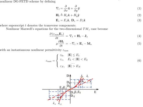
Figure 1. Linearization of the nonlinear constitutive relation.
The nonlinear constitutive relation can be linearized into several line segments by introducing the parametric variationalsλ. Take a five-segment approximation as shown in Fig. 1 as an instance, where E−1 =−E1,E−2=−E2,· · ·,E−N =−EN,D−1=−D1,D−2 =−D2,· · ·,D−N =−DN.
Assuming that 0< ε0 < ε1 < ε2 <· · ·< εN, let
where
λ1= (Dz−D1)
1 ε0 −
1 ε1
, Dz≥D1≥0
· · ·
λN = (Dz−DN)
1 εN−1−
1 εN
, Dz≥DN ≥0
λ−1 = (Dz−D−1)
1 ε1 −
1 ε0
, Dz≤D−1 ≤0
· · ·
λ−N = (Dz−D−N)
1 εN −
1 εN−1
, Dz≤D−N ≤0
λ=λ1+λ2+· · ·+λN −λ−1−λ−2− · · · −λ−N
(8)
Then we will have
λ≥0, λ1 ≥0, λ2 ≥0, · · · , λN ≥0
λ−1≥0, λ−2≥0, · · ·, λ−N ≥0
(9)
We will have
fi<0, if λi = 0; fi = 0, if λi >0, i=−N, . . . ,−1,1, . . . , N (10) Define
f1 =Dz−D1−λ1C1
· · ·
fN =Dz−DN −λNCN
f−1 =D−1−Dz−λ−1C−1
· · ·
f−N =D−N −Dz−λ−NC−N
C−1= ε1ε0
ε0−ε1, · · · , C−N
= εNεN−1 εN−1−εN
C1= ε0ε1
ε1−ε0, · · · , CN
= εN−1εN εN −εN−1
(11)
The constitutive relationships can be rewritten as f1<0, λ1 = 0; f1 = 0, λ1 ≥0
· · ·
fN <0, λN = 0; fN = 0, λN ≥0
f−1<0, λ−1= 0; f−1= 0, λ−1≥0
· · ·
f−N <0, λ−N = 0; f−N = 0, λ−N ≥0
(12)
Introducing slack variables vi to make above inequality become equations, the nonlinear constitutive
relations becomes
fi+vi= 0
λi ≥0, vi ≥0, λivi= 0 (13) We can see that treating nonlinearity is essentially solving a standard linear complementary problem (LCP) [13]. Several highly efficient computational methods [14–16] from computational mathematics can be used to solve the final quadratic programming model. Therefore, the iterative process in each time step is avoided in the proposed method. For a general nonlinear material, the nonlinear constitutive relation can be linearized into arbitrary number of line segments with a corresponding number of parameter variables, and the corresponding derivation of the equation can be referred to [12].
The corresponding parametric variationals weak forms of nonlinear Maxwell’s equations are
Si
ε0Ne·∂
(Ez+λ) ∂t ds =
Si
Ne· ∇t×Htds−
Si
Ne·Jsds (14)
Si
μNh·∂Ht
∂t ds = −
Si
Nh· ∇t×Ezds−
Si
where Ne and Nh are test-and-basic functions for Ez and Ht, respectively, and Si denotes the area of thei-th subdomain.
Using integration by parts and Gauss’s theorem in Equations (14) and (15), by applying some simple identities, we obtain
Si
ε0Ne·∂
(Ez+λ) ∂t ds =
Si
∇t×Ne·Htds−
Si
Ne·Js+
Li
Ne·(ˆn×Ht)dl (16)
Si
μNh·∂Ht
∂t ds = −
Si
∇t×Nh·Ezds−
Si
Nh·Ms−
Li
Nh·(ˆn×Ez)dl (17)
where nˆ is the outward unit normal of the boundary, and Li denotes the subdomain surface. The relationship of the interface fields between subdomainiand its neighbor subdomains can be evaluated as the two numerical fluxesˆn×Ez andˆn×Ht. As the basis functionsNeandNh are not required to be continuous across the interface between two adjacent subdomains, a nonconforming mesh can be used between subdomains. The Riemann solver [17–19] is used here to calculate the above numerical fluxes. Take thei-th subdomain as the local subdomain, and assume that it is adjacent to thej-th subdomain. The corrected fields on the interface will be
ˆ
n×Ez = ˆn×Y
iEi
z+YiEjz
Yi+Yj −nˆ×ˆn×
Hit−Hjt
Yi+Yj (18)
ˆ
n×Ht = ˆn×Z
iHi
t+ZiHjt
Zi+Zj +nˆ×ˆn×
Ezi −Ezj
Zi+Zj (19)
where Eiz and Hit are fields from the local (i-th) subdomain; Ejz and Hjt are from the neighbor (j-th) subdomain; and Z and Y are wave impedance and admittance of the medium
Zi= 1 Yi =
μi εi, Z
j = 1
Yj = μj
εj (20)
for thei-th andj-th subdomains, respectively.
The discretized system by the nonlinear DG-FETD method for the i-th subdomain is given in
Mieede
i
dt = K
i
eeei+Kiehhi+
j
Lijeeej+
j
Lijehhj−Ji−Mieedλ
i
dt (21)
Mihhdh
i
dt = K
i
heei+Kihhhi+
j
Lijheej +
j
Lijhhhj −Mi (22)
Mieemn =
Si
ε0Niem·Niends,
Mihhmn=
Si
μNihm·Nihnds (23)
Kieemn =
Li
Niem· {nˆ× nˆ×Nein}/Zi+Zjdl (24)
Kihhmn =
Li
Nihm· {nˆ× nˆ×Nhin}/Yi+Yjdl (25)
Kieh =
Si
∇ ×Niem·Nihnds+
Li
Niem· {nˆ×Nihn}Zi/Zi+Zjdl (26)
Kihemn =
Si
∇ ×Nihm·Niends+
Li
Nihm· {nˆ×Nien}Yi/Yi+Yjdl (27)
Lijeemn =
Li
Niem· {nˆ× nˆ×Nejn}/Zi+Zjdl (28)
Lijhh
mn =
Li
Nihm· {nˆ× nˆ×Njh
n}/
Lijeh
mn =
Li
Niem· {nˆ ×Njhn}Zi/Zi+Zjdl (30)
Lijhe
mn =
Li
Nihm· {nˆ×Njen}Yi/Yi+Yjdl (31)
Jim =
Si
Niem·Jsds, Mim=
Si
Nihm·Msds (32)
where ei and hi are vectors of the discretized electric and magnetic fields for the i-th subdomain; the matrices and vectors in Equations (21) and (22) have the same definitions as in [20]. As shown in Equations (21) and (22), a large system with small nonlinear regions can be divided into several smaller linear and nonlinear systems by this domain decomposition method. By doing this, we can solve the multi-scale system with small nonlinear regions efficiently using nonconforming meshes between the electrically fine and electrically coarse structures. The nonconforming meshes are used for the transition from nonlinear FETD meshes to linear FDTD grids in the hybrid method. Theoretically, the electrically fine structures can be divided into any number of subdomains with DGM in the proposed method. In this nonlinear hybrid FETD/FDTD method, we adopt the conventional linear FDTD scheme with the leap-frog scheme on a staggered Cartesian grid. The coupling between FDTD and nonlinear FETD is in the next section.
2.2. Coupling between the Nonlinear FETD and FDTD Methods
The discretized Equations (21) and (22) for nonlinear DG-FETD can be rewritten as a first order linear ordinary differential equation:
Mdφ
dt −Kφ=f−Γ dλ dt (33) where M= ⎡ ⎢ ⎢ ⎣
Miee 0 0 0 0 Mihh 0 0 0 0 Mjee 0 0 0 0 Mjhh
⎤ ⎥ ⎥
⎦, K=
⎡ ⎢ ⎢ ⎢ ⎢ ⎣
Kiee Kieh Lijee Lijeh Kihe Kihh Lijhe Lijhh Ljiee Ljieh Kjee Kjeh Ljihe Ljihh Kjhe Kjhh
⎤ ⎥ ⎥ ⎥ ⎥ ⎦ (34)
λ = λi λj T (35)
f = fi fj T (36)
Γ =
Γi 0 0 Γj
(37)
φ = ei hi ej hj T (38)
If the i-th subdomain does not contain nonlinear medium, Γi = 0. The Crank-Nicolson method can be used to solve this discretized first-order equations, and the simple central finite difference is used for the parameter vector λ. We will get a time stepping scheme as
(M−KΔt/2) ¯φn+1−(M+KΔt/2) ¯φn =
fn+1+fn
2 +Γ
λn+1−λn
dt (39)
subject to the LCPs equations
f(e, λ) +v= 0
vT ·λ= 0,v, λ≥0 (40) where ¯φn and ¯φn+1 are the values of fieldsφ at time steps tn and tn+1, respectively. We can see that
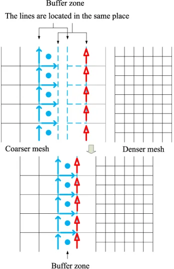
Figure 2. Coupling between coarser grid and denser grid with nonconforming mesh. The rectangular grid marked by dotted line is the buffer zone. The linear FDTD subdomain is on the left of the buffer, and the nonlinear FETD subdomain is on the right. Unknowns associated with edges marked by solid arrows,HF D, are exported from the linear FDTD grid to the nonlinear FETD mesh, and those marked
by empty arrows, HF E, are exported from the nonlinear FETD mesh back to the linear FDTD grid.
The EF D field is located at the cell center in the linear FDTD part marked by solid circle.
such as the aggregate-function smoothing algorithm can be used to solve Eq. (40) with high efficiency. Details of this algorithm can be referred to [15] and will not be elaborated here.
The edges of the explicit FDTD grid are updated using the FDTD scheme. This provides Equation (39) with a Dirichlet boundary condition [20]. The solution of Equation (39) is exported to the explicit grid to complete the full cycle of one time step (see Fig. 2). This process is repeated until the desired time window is completed.
For the example of 2-D TMz case, let us assume that En−1/2 and Hn are known in FDTD grid, and En andHn are known on nonlinear DG-FETD mesh, where the superscripts denote the time step index. To advance the fields to the next time step, we use the following procedures:
1. Use the FDTD method to advance the electric field toEn+1/2 with the known En−1/2 and Hn in the FDTD grid in Fig. 2.
2. Use the FDTD method to advance the magnetic field toHn+1 with the knownHn and En+1/2 in the FDTD grid in Fig. 2.
3. Pass HF Dn+1 components, marked by solid arrows in Fig. 2, from the FDTD grid to the nonlinear FETD buffer zone as the boundary values.
4. Use the Crank-Nicolson method to advance the fields in the nonlinear FETD subdomain fromn-th time step to (n+ 1)-th time step with the boundary values updated from FDTD in Step 3 above. After the solution of FETD subdomain for one full time step, the magnetic field values at the circles in Fig. 2, denoted byHF En+1, are known together with the other field values in the nonlinear FETD sub-domains.
6. Go to Step 1 and repeat the process until the specified time window has been reached.
The interfaces between adjacent subdomains can be nonconforming because the DG scheme permits discontinuous basis functions between adjacent subdomains. The elemental mass matrices for the rectangular linear edge elements in the buffer zone are obtained by the trapezoidal integration rule [20].
3. NUMERICAL RESULTS
3.1. Wave Propagation in 2D Structure with Nonlinearity
As shown in Fig. 3(a), the first example is about plane wave propagation in a rectangular zone inserted with one array of dielectric cylinders. The width and height of zone are 7.50 mm and 3.75 mm, respectively. The periodic boundary conditions [21] are applied to the upper and lower edges, and the perfectly matched layers [22] are used to truncate the computational domain along thex-direction. The radius of each dielectric cylinder is 0.164 mm, and the nonlinear relative permittivity isεr= 9.6+0.6|E|2. The lattice constants are both 0.492 mm along the x and y directions. This nonlinear problem is solved by both nonlinear FDTD method [6] and the proposed scheme. Fig. 3 shows the hybridization of FDTD grids and finite elements for the proposed scheme. The staggered Cartesian grid of Conventional FDTD (20∗40 cells) is used for the discretization of the homogeneous around the array of dielectric cylinders, and the unstructured element is applied to the zone filled with dielectric cylinders.
Discontinuous Galerkin technique is used to hybridize FDTD grid and unstructured element meshes. Nonconforming discretization is allowed on the interfaces between adjacent subdomains. This feature greatly improves the flexibility and efficiency of the proposed scheme in modeling the structures comprising of small nonlinear regions in an otherwise linear medium. An incident plane wave with transverse magnetic (TM) polarization is imposed at the left side of the computational domain. A receiver is located 1.875 mm away from the left boundary of the computational domain, and the time steps for the two methods are both 55 fs.
Figure 3. A rectangular zone filled with a array of dielectric cylinders.
Figure 4. Hybrid mesh for the nonlinear structure.
t(ps)
0 50 100 150 200 250
Ez(V/m)
-0.5 0 0.5 1 1.5 2 2.5
Benchmark FDTD with coarse grid FDTD with fine grid The proposed method
t(ps)
50 100 150
Ez(V/m)
-0.2 -0.1 0 0.1 0.2 0.3 0.4 0.5 0.6
Benchmark FDTD with coarse grid FDTD with fine grid The proposed method
t(ps)
0 50 100 150 200 250
Relative error
-0.06 -0.04 -0.02 0 0.02 0.04 0.06 0.08
FDTD with coarse grid FDTD with fine grid The proposed method
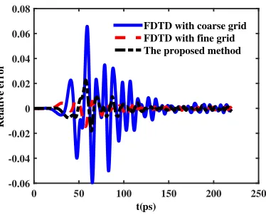
Figure 6. Time varying relative error by nonlinear FDTD and the proposed method.
(a) (b)
Figure 7. Electric field (V/m) near the dielectric circular rods at 0.0330 ns. (a) The proposed method, (b) nonlinear FDTD.
(a) (b)
Figure 8. Electric field (V/m) near the dielectric circular rods at 0.0495 ns. (a) The proposed method, (b) nonlinear FDTD.
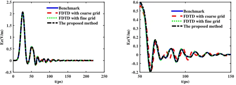
Figure 5 shows the simulated signals by the receiver for the two numerical techniques. The results obtained by nonlinear FDTD with a fine mesh (160∗320) are used here as reference. Good agreements can be observed between the results by the proposed method and nonlinear FDTD method. Fig. 6 shows the comparisons of relative errors by these two methods. From the figure we clearly see that the proposed scheme can achieve higher level of accuracy only by refining the mesh of nonlinear regions. Figs. 7–9 show the electric field near the dielectric circular rods at different times, and the results agree well with nonlinear FDTD and the proposed method.
(a) (b)
Figure 9. Electric field (V/m) near the dielectric circular rods at 0.0660 ns. (a) The proposed method, (b) nonlinear FDTD.
Table 1. Computational cost of the nonlinear FDTD and the proposed.
Coarse FDTD Fine FDTD The proposed method Benchmark
Grid 20*40 80*160 see Fig. 3 160*320
dt (fs) 55 55 55 55
Time length (ps) 220 220 220 220
Computational time (s) 14.53 256.46 161.22 1037.14
3.2. Nonlinear Structure with Multi-Subdomains
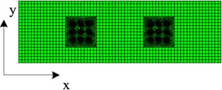
As shown in Fig. 10, the second example is about plane propagation in a rectangular zone inserted with two arrays of dielectric cylinders. The width and height of zone are 11.25 mm and 3.75 mm, respectively. The radius of each dielectric cylinder is 0.164 mm, and the nonlinear relative permittivity is εr = 9.6 + 0.6|E|2. The lattice constants are both 0.492 mm along the x and y directions. The separation of the two arrays is 3.75 mm.
The computational domain is meshed by an FDTD region outside (20∗65 cells), while the two arrays of dielectric cylinders are discretized by two subdomains with unstructured finite element meshes. Fig. 10 shows the structure of this case, which is decomposed into three subdomains discretized separately. The
Figure 10. A rectangular zone filled with two arrays of dielectric cylinders.
t(ps)
0 50 100 150 200 250
Ez(V/m)
-1 -0.5 0 0.5 1 1.5 2 2.5
Benchmark FDTD with coarse grid FDTD with fine grid The proposed method
t(ps)
50 100 150
Ez(V/m)
-0.6 -0.4 -0.2 0 0.2 0.4 0.6
Benchmark FDTD with coarse grid FDTD with fine grid The proposed method
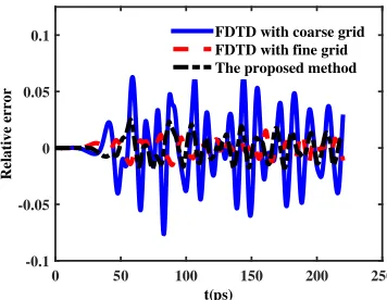
t(ps)
0 50 100 150 200 250
Relative error
-0.1 -0.05 0 0.05
0.1 FDTD with coarse grid
FDTD with fine grid The proposed method
Figure 12. Time varying relative error by nonlinear FDTD and the proposed method.
Table 2. Computational cost of the nonlinear FDTD and the proposed.
Coarse FDTD Fine FDTD The proposed method Benchmark
Grid 20*65 80*260 see Fig. 10 160*520
dt (fs) 55 55 55 55
Time length (ps) 220 220 220 220
Computational time (s) 25.05 418.91 328.75 1686.28
meshes could be nonconforming on the interfaces between adjacent subdomains. The nonlinear FDTD method and proposed method are used to solve this problem. A receiver is located 1.875 mm away from the left boundary of the computational domain, and the time steps for the two methods are both 55 fs. The results obtained by nonlinear FDTD with a fine mesh (160∗520) are used here as a benchmark. Fig. 11 shows the calculated signals by the receiver for nonlinear FDTD and the proposed method. Good agreements can be observed between the results by the proposed method and the benchmark, which demonstrate the validity of the proposed method with multi-subdomains. Fig. 12 shows the comparisons of relative errors by the nonlinear FDTD method and proposed method, and Table 2 shows the computational costs of the nonlinear FDTD and proposed method. We clearly see that the relative error of the proposed method is approximate to the FDTD with fine grid, but the computational time of proposed method is less.
4. CONCLUSIONS
We have demonstrated the validity of the nonlinear hybrid FDTD/FETD scheme by presenting numerical results for instantaneous nonlinear media. Using the parametric quadratic programming technique, this proposed scheme does not require updating system matrices and tedious iterative procedure at every time step. The proposed technique allows nonconforming meshes between different subdomains with linear and nonlinear media, making it suitable for structures comprised of small nonlinear regions in an otherwise linear medium.
ACKNOWLEDGMENT
This work is supported by the National Natural Science Foundation of China (Grant Nos. 51401045, 11502044 and 11472067) and Postdoctoral Science Foundation of China (Grant No. 2014M561222).
REFERENCES
2. Taflove, A.,Computational Electrodynamics: The Finite-Difference Time-Domain Method, Artech House, Norwood, MA, 1995.
3. Kunz, K. S. and R. J. Luebbers,The Finite Difference Time Domain Method for Electromagnetics, CRC, Boca Raton, FL, 1993.
4. Joseph, R. M. and A. Taflove, “Spatial soliton deflection mechanism indicated by FDTD Maxwell’s equations modeling,”IEEE Photonics Technology Letters, Vol. 6, 1251–1254, 1994.
5. Van, V. and S. K. Chaudhuri, “A hybrid implicit-explicit FDTD scheme for nonlinear optical waveguide modeling,”IEEE Transactions on Microwave Theory and Techniques, Vol. 47, 540–545, 1999.
6. Joseph, R. M. and A. Taflove, “FDTD Maxwell’s equations models for nonlinear electrodynamics and optics,” IEEE Transactions on Antennas and Propagation, Vol. 45, 364–374, 1997.
7. Ziolkowski, R., “Full-wave vector Maxwell equation modeling of the self-focusing of ultrashort optical pulses in a nonlinear kerr medium exhibiting a finite response time,”Journal of the Optical Society of America B, Vol. 10, 186–198, 1993.
8. Fisher, A., D. White, and G. Rodrigue, “An efficient vector finite element method for nonlinear electromagnetic modeling,”Journal of Computational Physics, Vol. 225, 1331–1346, 2007.
9. Chen, J., Q. H. Liu, M. Chai, and J. A. Mix, “A nonspurious 3-D vector discontinuous Galerkin finite-element time-domain method,”IEEE Microwave and Wireless Components Letters, Vol. 20, 1–3, 2010.
10. Zhu, B., J. Chen, W. Zhong, and Q. H. Liu, “A hybrid FETD-FDTD method with nonconforming meshes,”Communications in Computational Physics, Vol. 9, 828–842, 2011.
11. Tobon, L. E., Q. Ren, Q. T. Sun, J. Chen, and Q. H. Liu, “New efficient implicit time integration method for DGTD applied to sequential multidomain and multiscale problems,” Progress In Electromagnetics Research, Vol. 151, 1–8, 2015.
12. Zhu, B., H. Yang, and J. Chen, “A novel finite element time domain method for nonlinear Maxwell’s equations based on the parametric quadratic programming method,” Microwave and Optical Technology Letters, Vol. 57, 1640–1645, 2015.
13. Cottle, R. W. and G. B. Dantzig, “Complementary pivot theory of mathematical programming,” Linear Algebra Applications, Vol. 1, 103–125, 1982.
14. Ferris, M. C. and J. S. Pang, “Engineering and economic applications of complementarity problems,” SIAM Review, Vol. 39, 669–713, 1997.
15. Zhang, H. W., S. Y. He, and X. S. Li, “Two aggregate-function-based algorithms for analysis of 3D frictional contact by linear complementarity problem formulation,” Computer Methods in Applied Mechanics and Engineering, Vol. 194, 5139–5158, 2005.
16. Fischer, A., “A special Newton-type optimization method,”Optimization, Vol. 24, 269–284, 1992. 17. Lu, T., P. Zhang, and W. Cai, “Discontinuous Galerkin methods for dispersive and lossy Maxwell equations and PML boundary conditions,” Journal of Computational Physics, Vol. 200, 549–580, 2004.
18. Lu, T., W. Cai, and P. Zhang, “Discontinuous Galerkin time-domain method for GPR simulation in dispersive media,”IEEE Transactions on Geoscience and Remote Sensing, Vol. 43, 72–80, 2005. 19. Mohammadian, A. H., V. Shankar, and W. F. Hall, “Computation of electromagnetic scattering and radiation using a time-domain finite-volume discretization procedure,” Computer Physics Communications, Vol. 68, 175–196, 1991.
20. Zhu, B., J. Chen, W. Zhong, and Q. H. Liu, “A hybrid finite-element/finite-difference method with an implicit-explicit time-stepping scheme for Maxwell’s equations,” International Journal of numerical Modelling: Electronic Networks, Devices and Fields, Vol. 25, 495–506, 2012.
21. Luo, M. and Q. H. Liu, “Spectral element method for band structures of three-dimensional anisotropic photonic crystals,” Physical Review E, Vol. 80, 1–7, 2009.