Optimal Dynamic Resource Allocation in Activity Networks

(1)

Abstract

RAMACHANDRA, GIRISH A. Optimal Dynamic Resource Allocation in Activity Networks. (Under the direction of Professor Salah E. Elmaghraby).

We treat the problem of optimally allocating resources of limited availability under un-certainty to the various activities of a project to minimize a certain economic objective composed of resource cost and tardiness cost. Traditional project scheduling methods as-sume that the uncertainty resides in the duration of the activities. Our research asas-sumes that the work content (or “effort”) of an activity is the source of uncertainty and the dura-tion is the result of the amount of resource allocated to the activity, which then becomes the decision variable. The functional relationship between the work content (w), the resource allocation (x), and the duration of the activity (y) is arbitrary, though we assume that the relationship obeys the “power law.” In other words,y=f(w, xγ), where the exponentγ is some constant.

(2)

OPTIMAL DYNAMIC RESOURCE ALLOCATION

IN ACTIVITY NETWORKS

BY

GIRISH A. RAMACHANDRA

A DISSERTATION SUBMITTED TO THE GRADUATE FACULTY OF NORTH CAROLINA STATE UNIVERSITY

IN PARTIAL FULFILLMENT OF THE REQUIREMENTS FOR THE DEGREE OF

DOCTOR OF PHILOSOPHY

INDUSTRIAL ENGINEERING

RALEIGH MAY 2006

APPROVED BY:

DR. SUBHASHISGHOSAL DR. MATTHIASF. STALLMANN

DR. ABDELHAKIM ARTIBA DR. JAMESR. WILSON EXTERNAL COMMITTEE MEMBER

(3)

(4)

Biography

Girish Ramachandra was born on February 2nd, 1974 in Bangalore, India. He earned his Bachelors degree in Mechanical Engineering in 1995 from National Institute of Technology (formerly known as Karnataka Regional Engineering College) at Suratkal, India.

He then joined Larsen & Toubro group of companies, Mumbai, India, where he worked in their earth moving equipment manufacturing division for four years in production plan-ning and materials control.

In 1999, he joined North Carolina State University to pursue his graduate studies in Industrial Engineering, where he received his Masters degree in Industrial Engineering in 2002. During the period August 2001 to May 2002, he worked as a student research as-sociate with Logistics Management Institute, McLean, VA USA, in their Resource Analysis Group.

(5)

Acknowledgements

First and foremost, I thank Dr. Elmaghraby for his help, guidance, and support — financial, intellectual, and moral — during the course of my graduate study at NCSU. I consider myself very fortunate to have had the opportunity to work with him. I thank my committee members, Dr. Jim Wilson, Dr. Matt Stallmann, Dr. Ghosal, and Dr. Artiba for their insightful comments and for carefully reviewing my dissertation. I thank Dr. Lunardi for attending my preliminary and final exams as the graduate school representative. I am grateful to Dr. Fang and Dr. Nuttle for providing me with financial support at critical times during my graduate study. Thanks also to Cecilia for being such a wonderful graduate assistant.

I feel fortunate to have met a lot of nice people since arriving in Raleigh. Special thanks goes to Shashi Adiga, who made life a lot easier for me during the first few months. I will always appreciate his unflinching willingness to offer help and support. Thanks to Narahari for being such a fantastic person to live with. The last four years were memorable and I will definitely miss all the good times. Thanks to Abhinand and Shrini for their friendship and the wonderful times I spent hanging out with them. Thanks to all my friends — Harish, Gautam, Srivatsan, Bhavin, Srikant Nalatwad, Vinay, Rajasimhan, Raghuram, and many others — for making ‘Apt. 2512-201’ such a lively and entertaining place!

Thanks to my office mates Xiaoli, Sean, Yong, and others for their friendship and help. Special thanks to Burcu Özçam for being such a wonderful friend, and for all the help and support she provided during my stay at NCSU. Thanks also to Girish Kulkarni, Jawad, Sriram, Sridhar Dasu, Parikshit, and Akhil for being such good friends and peers — I enjoyed spending time with you guys!

(6)

to Vijay and Vaidehi for their friendship and wonderful hospitality.

I am extremely grateful to SAS Institute, Cary NC USA, for providing me financial sup-port through the last two years of my doctoral study. Special thanks to Radhika and Gehan for providing me the opportunity to work with them. I learned a lot during that time, and also made some good friends. Lindsey, Emily, Nilesh, Richard, Laura, Bengt, Balaji, and the rest of the SAS ORD group — thanks for the numerous enjoyable lunch-time (and office-time!) discussions.

(7)

List of Tables

2.1 Unimodal RCPSP Classification . . . 7

2.2 Multimodal RCPSP Classification . . . 8

3.1 Parameters of the Example Project. . . 18

3.2 Optimal solution—No Resource Constraints; Fixed Deadline. . . 20

3.3 Optimal Node Realization Times—No Resource Constraints. . . 20

3.4 Optimal Solution — Individual Resource Constraints. . . 21

3.5 Optimal Node Realization Times — Individual Resource Constraints. . . 21

3.6 Cutsets in the Example Project. . . 23

3.7 Optimal solution — Aggregate Resource Constraints. . . 27

3.8 Optimal Node Realization Times — Aggregate Resource Constraints. . . 27

3.9 Resource Allocation across theudc’s. . . 27

4.1 Values of Expected Total Cost for Fixed Allocations(x1, x2)and Varyingx3 . 45 4.2 Sample Output of LHS . . . 56

4.3 Data for Example Network 3. . . 57

4.4 Summary of Results for Project Completion Costs from Monte Carlo (MC) and LHS Runs . . . 59

4.5 P-deciles for the Resource Allocation Vector (Uniform (LHS) Case) . . . 59

4.6 Lower and Upper Bounds forWj . . . 62

(10)

List of Figures

3.1 Tardiness Cost Function. . . 17

3.2 Example Network 1. . . 19

3.3 Project withudc’s marked. . . 24

3.4 Comparison of Computation Times: R = 5, n = 20,T = 20, 40, 60, 80. . . 33

3.7 Comparison of Computation Times: R = 7, n = 50,T = 40, 60, 80. . . 34

3.8 Comparison of Computation Times:T = 40, n = 40,R= 7, 8, 9, 10. . . . 35

4.1 Example Network 2 and its State Space. . . 42

4.2 Surface Plot of Resource Allocations versus Total Cost. . . 46

4.3 Example Network 3. . . 52

4.4 Hierarchy of Cutsets (not a complete tree).. . . 53

(11)

Chapter 1 Introduction

1.1 Background

An important issue that looms high in the management of real life projects is that ofrisk anduncertainty. Concerns about risk are everyday worries of project managers. They rec-ognize the uncertainty in their estimates of resources, cost, and time. The issue is not about recognition, but aboutmeasurement(how does one measure the risk involved in a particular action), and aboutcopingwith uncertainty, especially in relation to resource allocation.

We are concerned with the concrete actions (decision making) relative to resource allo-cation to mitigate the deleterious effects of deviations, most of them unanticipated (known only in probability), in the progress of the project. In other words, suppose that the risk of a particular activity (or subset of activities) defaulting on its completion time (or cost estimate, or resource needs) is unacceptable, what can be done to reduce the risk, if not completely eliminate it?

1.2 Underlying Hypothesis

(12)

CHAPTER 1. INTRODUCTION

appreciable research and development content, in which the internal factors play the dom-inant role. Most importantly, even those studies that concerned themselves with the issues of resource allocation are marked by strict adherence todeterministicestimates of the var-ious parameters, ignoring (or skirting) the issue of uncertainty in the estimates of these parameters.

Uncertainty in the work content of an activity then is typically expressed by the manager in the form “it requires betweenl anduman-weeks” (where lis the lower bound and uis the upper bound), with or without knowledge of the probability distribution of the work content. In the face of such uncertainty in the work content the manager still has todecide on the resources to be devoted to the activity. The duration of the activity then becomes the consequenceof the resources allocated to the activity, not thesourceof the uncertainty.

This perspective changes the view of risk management in a radical fashion because now the decision is concerned with theoptimal resource allocation(with its concomitant cost) in order to achieve the desired objective; namely complete the project within the prescribed due date (in order to avoid any penalty of tardiness) and with minimal cost of resources.

We do not suggest that one ignore the external factors; indeed, they must be taken into consideration, sooner or later. But we wish to focus on the internal factors because the uncertainty stemming from them is the form of uncertainty that can be managedviaproper allocation of resourcesdynamically.

Thus our research has two pivotal elements that distinguish it from prior studies in this field. The first is that we consider uncertainty explicitly. And the second is that our take-off point is thework contentof the activity, not its duration.

1.3 Problem Statement

(13)

be the project due date, so that if the project completes at timetm1, then the total cost of tardiness would bect·max{0, tm−Ts}. Our objective is to optimally allocate resources to the activities such that the overall cost of resource allocation and tardiness is minimized.

1.4 Scope and Objectives of Research

The primary objective of this research is to address the problem of optimally allocating resources, that are limited in availability, to a project while minimizing a certain economic objective. the specific objectives can be summarized as follows:

1. Develop a mathematical model to solve the deterministic resource allocation problem when there are (a) unlimited resources, (b) resource availability constraints on indi-vidual resources, and (c) additional aggregate resource availability constraints across activities that can be performed in parallel.

2. Develop mathematical models that can address the stochastic version of the problem. Ideally, models that can be easily extended from the deterministic version.

3. Validate the mathematical models for correctness and robustness.

1.5 Organization of the Dissertation

The rest of this dissertation is organized as follows. The first part of Chapter 2 is a brief review of literature that describes the Resource-Constrained Project Scheduling Problem (RCPSP) and its variants, followed by some discussion on different methods used to solve them. It also draws attention to certain classes of problems that are similar to the problem addressed by our research. Chapter 3 discusses in detail the deterministic version of the resource allocation problem together with the two mathematical formulations — a non-linear programming (NLP) approach, based on the concept of uniformly directed cutsets (udc), and an integer programming (IP) model that is time-based. In Chapter4we address the stochastic version of the problem. We first discuss the Continuous-Time Markov Chain

(14)

(CTMC) approach when the work content of all activities are independent exponential ran-dom variables. We briefly outline the solution strategy and discuss the limitations of the approach in practice. The latter half of Chapter 4 is devoted to the case where the work content of activities follow a general probability distribution (i.e., not necessarily exponen-tial). The limitations of standard stochastic programming approach are discussed followed by details of the alternate approach of simulation-cum optimization. Efficient sampling methods to reduce sample size and sample variance are also described. Finally conclusions and recommendations for future research are outlined in Chapter5.

(15)

Chapter 2 Literature Review

This review is organized into three sections. In Section 2.1 we describe the Resource-Constrained Project Scheduling Problem (RCPSP) and its classification. In Section2.2we survey the work done on the unimodal and multimodal RCPSP. We are particularly inter-ested in themultimodalproblem mainly because it relates closely the concept ofwork con-tentadvocated here. We provide a review of the work done in the the variants of the RCPSP, including a brief discussion of the stochastic instance of the problem. Finally in Section2.3

we give an outline of the recent work done on the problem of optimal resource allocation in activity networks (Tereso et al. [2001, 2003b]).

2.1 Introduction and Classification of RCPSP

(16)

CHAPTER 2. LITERATURE REVIEW

of resource application, or several “substitutable" resources). Each mode implies a different option in terms of cost and/or duration. We broadly classify the RCPSP into the following six categories:

1. UnimodalRCPSP (SM–RCPSP)

2. MultimodalRCPSP (MM–RCPSP)

3. RCPSP with nonregular objective functions

4. Stochastic RCPSP

5. Multi–resource constrained Project Scheduling Problem (MRCPSP)

We focus on the first four items in our review. See Garey et al. [1976] for more on the relationship between RCPSP and the bin packing problem.

2.2 Unimodal and Multimodal RCPSP

(17)

1. minimization of weighted activity tardiness.

2. minimization of the total number of tardy activities.

3. minimization of weighted mean flow time.

Table2.1summarizes our classification ofunimodalRCPSPs. The Basic SM-RCPSP has been studied extensively in the literature. Typical solution strategies for this class of prob-lems are through mathematical programming techniques: integer programming and LP relaxation, combined with implicit enumeration (branch-and-bound), and dynamic pro-gramming.

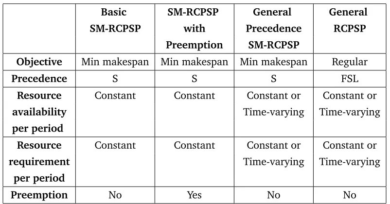
Table 2.1: Unimodal RCPSP Classification

Basic SM-RCPSP General General SM-RCPSP with Precedence RCPSP

Preemption SM-RCPSP

Objective Min makespan Min makespan Min makespan Regular

Precedence S S S FSL

Resource Constant Constant Constant or Constant or

availability Time-varying Time-varying

per period

Resource Constant Constant Constant or Constant or

requirement Time-varying Time-varying

per period

Preemption No Yes No No

A variety of branch-and-bound algorithms have been developed for this problem. Most use partial feasible schedules as a starting point and then extend them in the branching process until a complete schedule is found. Owing to the computational complexity of the RCPSP, several priority-rule-based heuristics have been proposed. For more details on the various branching and pruning strategies and heuristic approaches see Herroelen et al. [1998a].

(18)

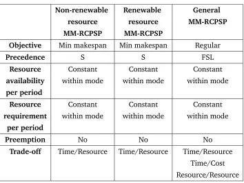
Table 2.2: Multimodal RCPSP Classification

Non-renewable Renewable General resource resource MM-RCPSP MM-RCPSP MM-RCPSP

Objective Min makespan Min makespan Regular

Precedence S S FSL

Resource Constant Constant Constant

availability within mode within mode within mode

per period

Resource Constant Constant Constant

requirement within mode within mode within mode

per period

Preemption No No No

Trade-off Time/Resource Time/Resource Time/Resource Time/Cost Resource/Resource

throughout the duration of the project.

In themultimodalRCPSP problem, a set of allowable execution modes can be specified based on the estimation of work contentof the activity. Each mode is characterized by a processing time and an amount of resource of a particular type needed for completion of the activity. A summary of classification of the multimodal RCPSP problems is shown in Table2.2. In the non-renewable–resource RCPSP, tasks are associated with non-renewable resources. A cost of resourcer while processing taski,ci(r), is associated with this mode. If the set of modes for every task can be represented as a closed interval and ci(r) is an affine and decreasing function of processing time pi, we have a linear time-cost trade-off problem. If the set has discrete values of ci(r) then we have a discrete time-cost trade-off (DTCT) problem.

(19)

that iteratively calculates a sequence of cuts in the AoA (Activity-on-Arc) network to com-pute the project cost curve. For the discrete case, the best known algorithms still rely on dynamic programming (DP), but additionally exploit the decomposition structure of the underlying network. All the reported algorithms for solving the DTCT problem exhibit ex-ponential worst-case complexity. A notable exception is the dynamic program by Hindelang and Muth [1997], which claimed to execute in pseudo-polynomial time. However De et al. [1997] demonstrate that the DP is flawed, and offer a simple correction. They further prove that the DTCT decision problem is stronglyN P–complete by reduction from the 3– SAT problem (see Garey and Johnson [1979]). Based on this result they imply that the DTCT optimization problem is stronglyN P–hard. As mentioned earlier, this class of mul-timodal RCPSP relates very closely to the problem of concern to us in this thesis, and we shall revisit it in Chapter3.

The renewable-resource RCPSP has been studied in some detail with respect to makespan minimization objective. Demeulemeester et al. [1997] present a branch-and-bound proce-dure based on the concept of maximal acivity-mode combination. An activity-mode combi-nation is a subset of activities executed in a specific mode; it is maximal if no other activity can be added without causing a resource conflict. Sprecher and Drexl [1998] developed a branch-and-bound procedure that relies on an enumeration scheme based on the “prece-dence tree" concept. Several heuristics have been developed as well; the recent genetic algorithm (GA) approach by Hartmann [1998] being worthy of note.

In the stochastic RCPSP, the processing time of any activity is a random variable (r.v.) that follows some probability distribution. This problem class, while more realistic, leads to much greater complexity in analysis. The commonly pursued objective is the minimiza-tion of the expected makespan. Since a project contains many interdependent activities, thereby leading to interdependent activity completion times, the probability distribution of the project completion time is extremely difficult to determine. Often it prompts the assumptions of independence for tractability of analysis. Such assumptions, however, can lead to extremely misleading results in practice.

(20)

constraint and the problem of achieving a feasible fixedexpectedproject completion time at minimum cost as well as generation of the project curve. Gutjahr et al. [2000] describe a stochastic branch-and-bound procedure for solving a specific version of the stochastic DTCT where so-called measures (like the use of manpower, the assignment of skilled labor, etc.) may be used to increase the probability of meeting the project due date, thereby avoid-ing penalty costs. Stork [2001] provides an excellent insight into the stochastic resource scheduling problem. He addresses the objective of makespan minimization and provides branch-and-bound algorithms. He uses the classicalcritical path lower bound and imple-ments some clever sorting rules, preselective policies, and dominance rules to prune the search tree. See the handbook by Demeulemeester et al. [1997] for more details.

(21)

was made). The work of Valls et al. [1998] provides a good example of application of stochastic programming to stochastic project scheduling under resource constraints. They deal with the problem of resource-constrained project scheduling with stochastic activity interruptions, where they minimize the total expected value of weighted tardiness. We discuss their problem in detail in section4.3.1of Chapter4.

2.3 Optimal Resource Allocation

The literature has been of little help on the problem of resource allocation in project net-works. Tereso et al. [2001, 2003a,b, 2004] deal with resource allocation in multimodal activity networks. They address the stochastic version of the problem and assume exponen-tial distribution for thework contentof activities.

(22)

fk(sk| F) denote the minimal cost at stagek when the state issk, and conditioned on the allocation inF. The DP functional equation is defined as

fk(sk|F) = min x[k]∈D

EC[k](x[k], sk) +E[fk−1(Sk−1| F)] ,

whereSk−1,ar.v., represents the realization time of statesk−1, k= 2, . . . , K.

The optimum is secured by removing the conditioning, and the final solution is achieved by evaluating the following:

f(sK= 0) = min

F fK(sK| F).

The solution obtained via dynamic programming yields a policy that prescribes the optimal resource allocation under every conceivable state of the project as it progresses over time.

The DP model just discussed is computationally very intensive. Just to get an idea, if there areq different allocation values of an activity in setF, and accordinglyq|F | possible allocations from which the optimum is selected. Tereso et al. [2003b] present some basic approximations to the DP model such as (i) replacing the work content of activities in the set

(23)

Chapter 3 Optimal Resource Allocation – Deterministic Case

In this chapter we discuss the scenario where the work content of each activity is determin-istic. We analyze three possible cases, namely

1. Unconstrained activities — Unlimited resources available

2. Individual resource constraints on activities — Resource usage for each activity is constrained between upper and lower bounds.

3. Aggregate resource constraints — In addition to individual resource constraints, the resource usage across different activities running in parallel at the same time is con-strained between upper and lower bounds. Resource(s) availability may be constant over time, or it may vary from period to period.

(24)

CHAPTER 3. OPTIMAL RESOURCE ALLOCATION – DETERMINISTIC CASE

that lead from one node to another. We define the termscutsetanduniformly directed cutset (udc)as follows:

Assume we have a graph G = (N, A), where N is the set of nodes and A is the set of arcs defining the activities and the precedence relations among them. LetB ⊂N andB¯ = N −B. Letiandi0 denote the start and end nodes of activityj, respectively. Furthermore, define B,B¯=j∈A:i∈B, i0 ∈B¯ .

Definition 3.1. The set of edges B,B¯is called an(s, t)-cut (or cutset) ifs∈B andt∈B¯.

Definition 3.2. An(s, t)-cutS ≡ B,B¯ is called a uniformly directed cutset (udc) if B, B¯

is empty. In other words, an(s, t)-cut is a udc if and only if no two arcs in the cut belong to the same path in the network.

3.1 Nonlinear Programming Model

We consider a very general model with more than one type of renewable resource. We incorporate general (nonlinear) functions for activity duration, resource usage cost and tardiness cost. For the sake of convenience we state the notation used as follows:

wj(r) : work content of activityj relative to resource typer; work content is typically expressed in units such as man-hours, man-days, machine-hours, etc.

xj(r) : amount of resource typer(men, machines, etc.) allocated to activityj yj(r) : duration of activityj corresponding to allocationxj(r)

Cj(R) : total cost of resource usage for activityj CR : total cost of resource usage for all activities CT : total cost of tardiness

Note: If only one type of renewable resource is available, one can simply use the nota-tions wj, xj, and yj to refer to work content, resource allocation, and activity duration, respectively.

3.1.1 Unconstrained Activities

(25)

of abundant availability, at a price, of course. The duration of the activity, yj(r) can be modeled as a function of the resources allocated to it as

yj(r) = wj(r)

xγ_j(r), (3.1)

where the exponent γ is constrained to be γ ∈ [0.5,1.0]. For instance, if γ = 0.5, then doubling the resource allocation will decrease the duration by only about 30%,

y2 y1

= w/

√

2x (w/√x) =

1

√

2 = 0.707. On the other hand, ifγ = 0.75,then

y2 y1

= 1

20.75 = 1

1.68 = 0.59,

which means that the duration is reduced by about 41%, etc. Typically one would encounter such functional relationship between resource allocation and resulting duration in software development projects. Observe that ifγ >1(representing synergism) then one can achieve super-linear improvement in duration by increased resource allocation.

The duration of the activity, denoted byyj,is themaximumof the individual durations secured from each resource,

yj = max{yj(r)}_r=1,2.

Since it does not make sense to incur cost unnecessarily due to excessive resource allocation, it must be true that (taking note of (3.1)),

yj(r1) = wj(r1) xγ1

j (r1)

= wj(r2) xγ2

j (r2)

=yj(r2),

and hence,

xj(r2) =

wj(r2) wj(r1)

1

γ₂

x

γ₁ γ₂

j (r1). (3.2)

One may perform a data pre-processing step to calculate the ratios

wj(r2) wj(r1)

1

γ₂

and γ1 γ₂, which are denoted byφ_j andγ_1,2, respectively. In other words,

φ_j =

wj(r2) wj(r1)

1 γ₂

(3.3)

γ_1,2 = γ1

(26)

Henceforth one may speak ofxj(r2)in terms ofxj(r1)to yield the same duration,

xj(r2) =φjx γ1,2

j (r1). (3.5)

Likewise,yj can be expressed in terms of resourcer1 only,

yj =wj(r1)·x−jγ1(r1). (3.6)

The activity’s cost of resources usage,Cj,Rassumes the following form:

Cj(R) = X

r=1,2

kj(r)x2j(r)·yj (3.7)

in whichkj(r) is a constant of proportionality which may vary with the activityj and the resourcer. Note that we also assume the resource usage cost (for both types of resources) to be quadratic in the duration of the activity, hence the exponent 2 forxj(r). It is possible that it could vary with resource r and activity j. Substituting for yj from (3.6) and for xj(r2)from (3.5) into (3.7) we get,

Cj(R) = kj(r1)·x2_j(r1)·yj+kj(r2)·x2_j(r2)·yj = yj

kj(r1)·x2j(r1) +kj(r2)·

φ_jxγ1,2

j (r1) ₂

, (3.8)

a function of onlyxj(r1).

The total cost of both resources (recall that we are assuming only two resources) is simply the sum ofCj(R)over all the activities

CR= X

j∈A

Cj(R). (3.9)

We are now ready to deal with the cost of tardiness. To this end we assume that the project has a specified due dateTs,and that the cost of tardiness ispiecewise linearand con-vex in the tardiness1, with slopesp1 < p2 <· · · . (This can be used to closely approximate any convex nonlinear function of tardiness.) Assuming that the project is completed at time tm, the total cost of tardiness is given by,

CT =       

p1(tm−Ts), ifTs≤tm≤b1, p1(b1−Ts) +p2(tm−b1), ifb1≤tm≤b2,

etc.

(3.10)

1 _{An incentive for completing the project before the specified time}_T

s can be easily incorporated into the

(27)

ΤΤΤΤ_s _b

1 b2

slope p3

slope p2

slope p₁

t_n

T

ar

din

es

s

C

os

t,

CT

Due date

Figure 3.1: Tardiness Cost Function.

The costing of tardiness would appear as shown in Fig.3.1.

Based on these assumptions it is easy to see that the objective is to determine the allo-cation vectorX∗that achieves:

min

X z(X) =CR+CT (3.11)

The only “structural" constraints we have to deal with are the precedence constraints. Lettidenote the time of realization of nodei, with the assumption thatt1 = 0(the project starts at time 0) and the nodes in the AoA representation of the project are numbered topologically so that an arrow always leads from a smaller number to a larger one. Then the realization of nodemsignals the completion of the project. We have,

ti0 ≥ti+yj, ∀j≡ i, i0

∈A. (3.12)

Total tardiness is defined asv= max{0,(tm−Ts)}, which is replaced by the constraint

v≥tm−Ts, (3.13)

together with the requirement thatv≥0.

Finally we have the nonnegativity constraints,

(28)

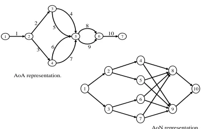
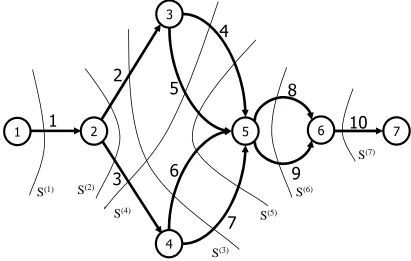
We now consider the “logical" constraints imposed by the nature of the problem, which stem from the desire to equate the durations of paths in parallel. Consider an example network shown in Figure3.2. We have,

Activities 4 & 5 are in parallel : y4=y5 (3.15) Activities 6 & 7 are in parallel : y6=y7 (3.16) 2 parallel paths†from node 2 to node 5 : y2+y4 =y3+y6 (3.17) Activities 8 & 9 are in parallel : y8=y9 (3.18)

†_{A path is identified by the activities on it.}

The mathematical program defined by the objective of Equation (3.11) with its variables defined in Equations (3.5)–(3.10), and constraints (3.12)–(3.18) is the desired model for this problem.

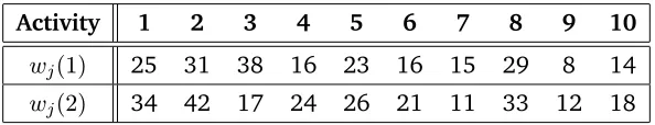
Consider the project network shown in Figure3.2with values of the various parameters as given in Table 3.1. The work content is measured in man-days. The due date Ts = 36,with tardiness cost cut-off pointsb1 = 5, b2 = ∞,and slopesp1 = 200, p2 = 800.The interpretation of the pair (b2 = ∞,p2 = 800) is that beyond the cut-off pointb1 = 5, the tardiness is penalized at the rate of 800. The resource usage coefficients (exponents for xj(r) in (3.7)) are 1.5 for resource 1 and 2 for resource 2. The resource coefficients are γ_j(1) = 0.90, γ_j(2) = 0.95, the same for all activities. The resource cost coefficients are also the same for all activities, withkj(1) = 6, kj(2) = 8.

Table 3.1: Parameters of the Example Project.

Activity 1 2 3 4 5 6 7 8 9 10

wj(1) 25 31 38 16 23 16 15 29 8 14 wj(2) 34 42 17 24 26 21 11 33 12 18

The optimal solution (obtained using AMPL/MINLP-BB2_{on NEOS}3_{optimization server)}

to this set of parameters is as shown in Table3.2. The corresponding node realization times

2_{See Fletcher and Leyffer [1998] and Leyffer [2001] for details on the MINLP-BB algorithm.}

3_{See Czyzyk et al. [1998], Gropp and Moré [1997], Dolan [2001] for details on the NEOS Optimization}

(29)

7 6

5

4 3

2

1 1 10

2

3

4

5

6

7 8

9

AoN representation. The graph is s/p.

10

9

7 6 5 4

3

2 8

1

AoA representation.

Figure 3.2: Example Network 1.

are shown in Table3.3. Observe that the optimal solution reached, but did not exceed, the cut-off value ofb1= 5,mainly due to the very high cost of tardiness beyondb1= 5.

3.1.2 Individually Constrained Activities

We continue to assume that we know deterministically thework contentwj for each activity in the project, that we have only two resources to contend with, and that the work content of activityj relative to the two resources are denoted bywj(r),r = 1,2. The definition of the the variables remains as before, together with the costing relative to resource usage and tardiness.

But now we assume that the amount of each resource allocated to the activity is indi-vidually constrained,

(30)

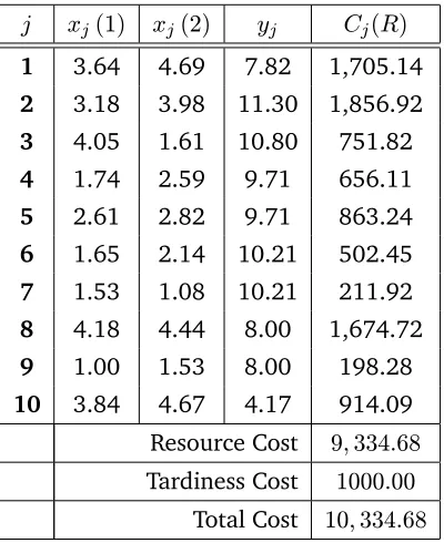
Table 3.2: Optimal solution—No Resource Constraints; Fixed Deadline. j xj(1) xj(2) yj Cj(R)

1 3.64 4.69 7.82 1,705.14

2 3.18 3.98 11.30 1,856.92

3 4.05 1.61 10.80 751.82

4 1.74 2.59 9.71 656.11

5 2.61 2.82 9.71 863.24

6 1.65 2.14 10.21 502.45

7 1.53 1.08 10.21 211.92

8 4.18 4.44 8.00 1,674.72

9 1.00 1.53 8.00 198.28

10 3.84 4.67 4.17 914.09 Resource Cost 9,334.68 Tardiness Cost 1000.00

Total Cost 10,334.68

Table 3.3: Optimal Node Realization Times—No Resource Constraints.

Node,i 1 2 3 4 5 6 7

Time,ti 0 8 19 19 29 37 41

The rationale for such bounds may run as follows. The lower bound may represent the least amount of resource needed to “get the activity going," or the least amount of resource acquisition possible (e.g., you cannot rent a truck for less than half a day), and the upper bound may represent the maximal allocation that the activity can bear, or the maximal availability of the resource in the marketplace, etc.

We now have two types of constraints: precedence constraints and resource constraints. The precedence constraints are the same as discussed earlier and shall not be repeated, see (3.12). The resource constraints are as defined in (3.19). Equation (3.13) defines tardiness. Finally, we have the nonnegativity constraints (3.14). The mathematical program is the same as in Section3.1.1, but with the addition of constraints (3.19).

(31)

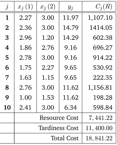
Table 3.4: Optimal Solution — Individual Resource Constraints. j xj(1) xj(2) yj Cj(R)

1 2.27 3.00 11.97 1,107.10

2 2.36 3.00 14.79 1414.05

3 2.96 1.20 14.29 602.38

4 1.86 2.76 9.16 696.27

5 2.78 3.00 9.16 914.22

6 1.75 2.27 9.65 530.92

7 1.63 1.15 9.65 222.35

8 2.76 3.00 11.62 1,156.81

9 1.00 1.53 11.62 198.28

10 2.41 3.00 6.34 598.84

Resource Cost 7,441.22 Tardiness Cost 11,400.00 Total Cost 18,841.22

Table 3.5: Optimal Node Realization Times — Individual Resource Constraints.

Node,i 1 2 3 4 5 6 7

Time,ti 0 12 27 27 36 48 54

Figure3.2. The parameters are the same as in Table3.1with the following modification — each activity j has bounds[lj(r), uj(r)]on the amount of resource r that can be allocated to it. For simplicity of exposition we assumed[lj(r), uj(r)] = [1,3]for all activitiesj ∈ A, and for both resources,r = 1,2. The optimal solution to this set of parameters is shown in Table3.4.

(32)

54 time units.

Whenever the resource allocation for an activity is between its bounds it corresponds to the optimal allocation either absolutely (relative to its resource cost) or conditional upon minimizing the tardiness cost. For instance, consider activity 1. Its resource cost is

C1(R) = y1 6x1.5₁ (1) + 8x2₁(2)

=

6x1.5₁ + 8

(w1(2)/w1(1))(1/γ2)×xγ11/γ2(1) ₂

×

w1(1) xγ1

1 (1)

= 150x0.60₁ (1) + 382.09x0.9947₁ (1),

a function of onlyx1(1),which is minimized atx1(1) = 1,its lower bound. However, this would prolong the duration of activity 1 from its current value of 11.97 to ≈ 25. This, in turn, would prolong the completion time of the project by 13 units, assuming that other activities remain the same(= 25−11.97), costing an additional13×800≈10,400.

3.1.3 Aggregate Resource Constraints

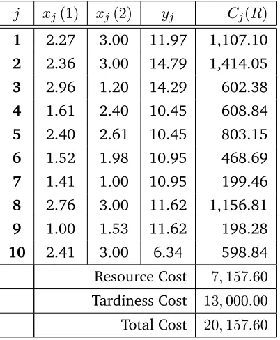
We now address the most general model of this genre of problems in which, in addition to the bounds on individual resource usage for each activity, there is also an aggregate constraint on the total resource usage at any time. This constraint is present whenever the resource availability is limited. This scenario is akin, but not identical, to the RCPSP. The most important distinction is the concept of work content and the focus on obtaining optimal specification of the resource allocation to the activities. We submit that this is a more realistic scenario which reflects the managerial discretion in resource allocation. Further, our scenario can easily accommodate the classical RCPSP scenario by defining discrete values of possible resource allocations and its variants.

The variables, parameters, and constraints of the model in Section3.1.2 remain intact in the model proposed here. But the introduction of the condition that at any time no more than the available capacity of each resource is utilized gives rise to the consideration of two aggregate capacities R1 and R2 (recall that we are still assuming that there are only two resources) so that the total resource allocated to anyconcurrentactivities at any timetis at mostRr.This may be written generically as,

X

concurrent

(33)

There remains the definition of “concurrent" activities, for which we must appeal to the concept ofuniformly directed cutset(udc), which has a long and venerable history (see Her-roelen et al. [1998a] for a summary review).

It is intuitively clear that at any time, progress in the project must be along activities that lie on audc. The first reaction to this realization is to enumerate alludc’s and constrain the total resource usage in each one. But slight reflection reveals that such blanket cover-age may result in anover-constrainedmodel, mainly due to the possibility that an activity, or several activities, may have already completed their processing and they are no longer involved in the “current"udc. In which case, including the completed activities in the con-straint for the new udc would then limit the resources available to the newly introduced activities, possibly resulting in a higher cost.

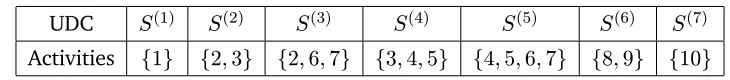
To fully comprehend the impact of such over-constraining, consider the example net-work of Figure 3.2, re-drawn in Figure3.3with all the udc’s displayed. In all, there are 7 udc’s, as shown in Table3.6below. We use the notationS() to denote audc. When we use the prefixcutsetwithS(), we are actually referring to theudc.

Table 3.6: Cutsets in the Example Project.

UDC S(1) S(2) S(3) S(4) S(5) S(6) S(7) Activities {1} {2,3} {2,6,7} {3,4,5} {4,5,6,7} {8,9} {10}

Suppose that progress is on-going on activities 2 and 3 in S(2) (referred to as activities 2 and 3 being “active"), and suppose activity 2 finishes first. Then activities 4 and 5 can be initiated and “control" moves tocutset S(4).To be sure, the total resource usage was first constrained by

X

j∈S(2)

xj(r)≤Rr, r= 1,2,

and then by

X

j∈S(4)

xj(r)≤Rr, r= 1,2.

(34)

7

6

5

4

3

2

1

10

2

3

4

5

6

7

8

9 S

(1)

_S

(2)

S

(3)

S

(4)

S

(5)

S

(6)

S

(7)

Figure 3.3: Project withudc’s marked.

S(5), which gives rise to the constraint, X

j∈S(5)

xj(r)≤Rr, r= 1,2.

Observe thatcutsetS(3) ={2,6,7}never appeared, and its corresponding constraint X

j∈S(3)

xj(r)≤Rr, r= 1,2

did not play any role in the definition of the resources allocated to any of the 6 activities 2,3,4,5,6,7! Taking such constraint into account would have “over-constrained" the allo-cation because the alloallo-cation to activity 2 may have been high, which would drastically confine the allocation to activities 6 and 7. A similar analysis can be made for the case in which activity 3 finishes first, or when both activities finish “almost at the same time."

(35)

cutset S(2), and that cutset S(3) will be the “controlling" cutset if activity 3 finishes first; cutset S(4) will be the “controlling"cutset if activity 2 finishes first; andcutset S(5) will be the “controlling" cutset if activities 2 and 3 finish “at the same time," or almost so. This translates into the following condition:

ift4 ≤t3−ε : S(2)→S(3) else if,t3 ≤t4−ε : S(2)→S(4) else,|t3−t4|< ε : S(2)→S(5)

(3.21)

In the above conditionεis some minimal spacing in time between the realization of the two nodes to be considered having been realized at different times.

This logic translates into the following set of constraints in whichδ(·)andρ(·)are binary 0,1 variables, andM is a large number.

t3−t4 ≤ −ε+M δ(3,4) (3.22) t4−t3 ≤ −ε+M ρ(3,4) (3.23) t3−t4 ≤ −ε+M

1−δ(3,4)+ρ(3,4)

(3.24) t4−t3 ≤ −ε+M

1 +δ(3,4)−ρ(3,4)

(3.25) t3−t4 ≤ ε+M

2−δ_(3,4)−ρ_(3,4)

(3.26) t4−t3 ≤ ε+M

2−δ(3,4)−ρ(3,4)

(3.27) X

j=3,4,5

xj(r) ≤ Rr+M

1−δ_(3,4)+ρ_(3,4)

, r= 1,2 (3.28) X

j=2,6,7

xj(r) ≤ Rr+M

1 +δ(3,4)−ρ(3,4)

, r= 1,2 (3.29) X

j=4,5,6,7

xj(r) ≤ Rr+M

2−δ(3,4)−ρ(3,4)

, r= 1,2 (3.30)

(36)

δ_(3,4) ρ_(3,4) Consequences

0 0 cannot be realized

0 1 (3.25), (3.29) are constraining 1 0 (3.24), (3.28) are constraining

1 1 either (3.26) or (3.27), and (3.30) are constraining

The reason why the (0,0) eventuality cannot be realized is that having both variables equal to 0 would cause inequality (3.22) to impose the constraint

t3 ≤t4−ε

which would contradict inequality (3.24), which says that

t3 ≥t4+ε.

Therefore one of the three conditions specified in (3.21) must be realized. The condition t3 < t4−εis satisfied by the pair(1,0)and constraint (3.24), and the conditiont4 < t3−εis satisfied by the pair(0,1)and constraint (3.25); finally the condition|t3−t4|< εis satisfied by the pair(1,1)and constraints (3.26) and (3.27). The respective resource constraints of (3.28)–(3.30) perform the desired restrictions on the resource allocation accordingly.

The above analysis reveals the difficulty in the implementation of this model. A set of nine constraints similar to (3.22)–(3.30), involving the definition of two binary variables, must be written for every pair of parallel nodes. The illustrative example of Figure3.2was selected advisedly because it manifests all the characteristics of larger projects and yet is small enough that it can be solved to optimality.

For illustrative purposes the model was solved to optimality assuming total availability of R1 = 8, R2 = 8, and ε = 0.50. The aggregate resource constraints, R1 and R2 were chosen in such a way that at least one of the constraints (3.20) is binding. Table3.7has the solution.

Activity 2 actually finishes at t3 = 26.76,and activity 3 finishes at t4 = 26.26;both are rounded off to 27 in Table3.8. Since we assumed the minimal spacing ε= 0.5for which the activities are considered to have completed at different times, and since the difference

(37)

Table 3.7: Optimal solution — Aggregate Resource Constraints. j xj(1) xj(2) yj Cj(R)

1 2.27 3.00 11.97 1,107.10

2 2.36 3.00 14.79 1,414.05

3 2.96 1.20 14.29 602.38

4 1.61 2.40 10.45 608.84

5 2.40 2.61 10.45 803.15

6 1.52 1.98 10.95 468.69

7 1.41 1.00 10.95 199.46

8 2.76 3.00 11.62 1,156.81

9 1.00 1.53 11.62 198.28

10 2.41 3.00 6.34 598.84

Resource Cost 7,157.60 Tardiness Cost 13,000.00 Total Cost 20,157.60

Table 3.8: Optimal Node Realization Times — Aggregate Resource Constraints.

Node,i 1 2 3 4 5 6 7

Time,ti 0 12 27 27 38 49 56

Table 3.9: Resource Allocation across theudc’s. UDC Resource 1 Resource 2

(38)

time, for all practical purposes. This is verified by the fact that both δ(3,4) and ρ(3,4) are equal to 1. Therefore the controlling cutset (see Fig. 3.3) is S(5) = {4,5,6,7}, and the constraining equations are (3.26), (3.27), and (3.30). The above table indicates that the total requirements for thiscutsetof resource 1 is≈6.94and for resource 2 is≈7.99.This is in line with our assertion earlier.

3.1.4 Limitations of the NLP Model

As seen in the case of aggregate constraints, one needs to identify nodes that are in “parallel” and then impose a set of 9 constraints similar to (3.22)–(3.30) for each pair. But in general, if there areppaths in parallel, each containingknodes, there shall be9k p₂= 9kp(p−1)/2 such constraints involving the definition of kp(p−1)integer-valued variables. Of course this is in addition to the constraints of the model specified in Section3.1.2, some of which are nonlinear.

(39)

3.2 Integer Programming Formulation

The biggest drawback of the NLP formulation, as alluded to earlier, is that it cannot be used when the underlying project network is not series/parallel. We therefore shift our focus to “time interval-based” monitoring of resources as opposed to “cutset-based” approach in the NLP model. In other words, we have an integer program which incorporates discrete-time indexing of variables that correspond to resource usage.

We now restate our problem in the context of a single-type renewable resource availabil-ity. We are given a projectG= (N, A), whereN = (1,2, . . . , m)nodes andA= (1,2, . . . , n) activities. Each activityj∈Ahas a work contentwj. Denote byxk, the amount of resource in mode kallocated to an activity, and c·xk, the resulting resource utilization cost. Note thatcis just a coefficient. The duration of of an activity is defined asyjk =wj/xk. LetTsbe the overall project due date, and letct be the cost of tardiness per unit of delay. The total cost of tardiness is defined asct·max{0, tm−Ts}, wheretm is the completion time of the project. Finally, letRtdenote the availability of resource in periodt.

We now proceed with the formulation of the integer program. Define two binary vari-ables, β_jt and δjt, corresponding to every (i, i0) ∈ A. Also define the following binary variables:

αjkt =  



1 : if activityjisactivein modekin periodt 0 : otherwise

zjk =  



1 : if activityjis executed in modek 0 : otherwise

Define integer-valued variables as follows:

• sj: start time of activityj

• fj: finish time of activityj

• ti: time of realization of nodei

(40)

CHAPTER 3. OPTIMAL RESOURCE ALLOCATION – DETERMINISTIC CASE min X j X k

zjk(c·xk·wj) +ct·max{0, tm−Ts} (3.31)

subject to

sj ≥ ti, ∀j ≡(i, i0)∈A (3.32)

fj ≥ sj+ K X k=1 zjk wj xk

, ∀j (3.33)

ti0 ≥ fj, ∀j≡(i, i0)∈A (3.34)

K X

k=1

zjk = 1, ∀j∈A (3.35)

αjkt ≤ zjk, ∀j∈A, ∀t∈ T, ∀k (3.36) X

j X

k

αjktxk ≤ Rt, ∀t∈ T (3.37)

X

k

αjkt ≤

t−sj

T + 1, ∀j∈A, ∀t∈ T (3.38)

X

k

αjkt ≤

fj−t

T + 1, ∀j∈A, ∀t∈ T (3.39)

β_jt ≥ t−sj

T , ∀j∈A, ∀t∈ T (3.40)

δjt ≥

fj−t+ 1

T , ∀j∈A, ∀t∈ T (3.41)

X

k

αjkt ≥ βjt+δjt−1, ∀j ∈A, ∀t∈ T (3.42)

s, t ≥ 0,integer (3.43)

αjkt, βjt, δjt ∈ {0,1} (3.44)

The objective function (3.31) is composed of total resource cost and tardiness cost4_.

Constraint (3.32) and (3.33) define the start and finish times of activity j, respectively. Constraint (3.34) defines the realization time of nodei0, ∀(i, i0) ∈ A. Constraint (3.35) ensures each activityjuses exactly one mode of the resource. Constraint (3.36) maintains consistency between variables αjkt and zjk in terms of resource mode chosen. Finally, Constraint (3.37) enforces resource constraints for every periodt.

4_{The term}_c

(41)

Consider the constraints (3.38)–(3.42), which are defined for each combination of time tand activityj. By definition of T, both t−sj

T and fj−t

T lie in the interval [-1, 1]. Now consider the following three cases:

1. Ift≤sj −1, then

• LHS of (3.38)<1, forcingαjkt to be 0

• (3.39) and (3.40) are non-binding

• (3.41) forcesδjtto be 1

• (3.42), along withαjkt= 0, forcesβjtto be 0

2. Ift≥fj+ 1, then

• LHS of (3.39)<1, forcingαjkt to be 0

• (3.40) forcesβ_jt to be 1

• (3.42), along withαjkt= 0, forcesδjt to be 0

3. Ifsj ≤t≤fj, then

• (3.40) and (3.41) force bothβ_jtandδjtto be 1

• (3.42) now forcesαjktto be 1

3.3 Setup of Computational Experiments for the IP Formulation

(42)

We classify the computational experiments into the following categories:

Category 1: Fix the work content of all activities, the value of resource availability (R), and the available modes to choose from. For each value of n — that is, the number of activities — repeat the experiment for

(a) different values of complexity index (CI) of the network, and

(b) different values of the upper bound on the project completion time(T).

Category 2:Fix the upper bound on the project completion time (T) and the number of activities (n). Repeat the experiment for

(a) different values of resource availability (R), and

(b) different values of complexity index (CI) of the network.

The results in Category 1 shed light on how the performance of the optimization of the IP is affected with the increase in the size and complexity of the project network. The results in Category 2 help us in learning how the performance of the IP optimization is affected with the restrictiveness of the resource availability. The computational results are reported in the following sections.

3.3.1 Computational Results: Category 1

We report the computation times for the following problem parameters: (i) R= 5, resource modes = { 1, 2, 3 },n= 20, 30

(ii) R= 7, resource modes = { 1, 2, 3 },n= 40, 50

The resource availability was increased from5to7forn= 40 andn= 50 for the following reason: the restrictiveness of the resource availability coupled with the increase in number of activities renders the IP infeasible. We have to either reduce the work content of the activities or increase the upper boundT.

(43)

0 100 200 300 400 500 600

20 40 60 80

Upper Bound on Completion Time (T) Tim

e ( se c)

CI = 2 CI = 3 CI = 4 CI = 5

Figure 3.4: Comparison of Computation Times: R = 5, n = 20,T = 20, 40, 60, 80.

0 100 200 300 400 500 600 700 800

20 40 60 80

e ( se c)

CI = 2 CI = 3 CI = 4 CI = 5

(44)

0 100 200 300 400 500 600 700 800

20 40 60 80

e ( se c)

C=2 C=3 C=4 C=5

Figure 3.6: Comparison of Computation Times: R = 7, n = 40,T = 20, 40, 60, 80.

0 200 400 600 800 1000 1200 1400

40 60 80

e ( se c)

CI = 2 CI = 3 CI = 4 CI = 5

(45)

3.3.2 Computational Results: Category 2

In order to observe the performance of the IP with relaxing the resource availability, we chosen= 40,T = 40 and varied the resource levelRfrom 7 to 10 in increments of 1. As seen from Fig. 3.8, the computation time drop drastically asR increases. The decrease is steeper in networks with higher CI (4 and 5) mainly because of more parallel paths in the network.

0 100 200 300 400

6 7 8 9 10 11

resource availability (R)

Tim e ( se c)

CI = 2 CI = 3 CI = 4 CI = 5

Figure 3.8: Comparison of Computation Times: T = 40, n = 40,R= 7, 8, 9, 10.

3.3.3 Observations from Computational Experiments

(46)

Chapter 4 Optimal Resource Allocation – Stochastic Case

In this chapter we study the optimal resource allocation to the activities of a project in or-der to optimize an economic objective in the face of uncertainty. In Section 4.1 we state our problem along with the assumptions. In Section 4.2we outline a Policy Iteration–like procedure for solving such networks. We model it as a Continuous-Time Markov Chain on the lines of the work by Kulkarni and Adlakha [1986] and we proceed to introduce the phase type distribution that plays an important role in the policy evaluation. In Section4.3

we outline the technique of stochastic programming (SP), which is also known as mathe-matical programming under uncertainty. We discuss a recent research effort that applies the concept of SP to a stochastic resource-constrained project scheduling problem. Follow-ing that discussion, we demonstrate the inapplicability of standard SP techniques to our problem. Finally in Section 4.4we describe a simulation-cum optimization technique that implements variance reduction techniques (VRT) in order to reduce the sample size and the sample variance. We illustrate the effectiveness of the VRT implemented with the help of an example, and also briefly describe how the output data of the simulation experiment can be used to address related problems of interest.

4.1 Problem Statement and Assumptions

(47)

CHAPTER 4. OPTIMAL RESOURCE ALLOCATION – STOCHASTIC CASE

renewable resource and letxj be the allocation of the resource to activity j. AssumeR as the total availability of the renewable resource in any period. Definecr to be the per-unit cost of usage of resource per unit time. We further assume that the project has a specified due date Ts, a constant, and let ct(max{0,Υ−Ts}) be the cost of tardiness when the project completes at timeΥ, a random variable. Our objective is to determine the resource allocation vector,Xto the activities such that the overallexpectedcost of resource allocation and tardiness is minimized.

4.2 Policy Iteration–like Approach

For the sake of tractability in analysis, assume that the activity’s work content,Wj, a random variable, follows an exponential distribution

Wj ∼Exp(λj), ∀j∈A.

Assume that the resource allocationxj is bounded from above and below as:

0≤lj ≤xj ≤uj <∞, ∀j∈A.

Let the resulting duration of activityj,

Yj = Wj

xj ,

It is clear that Yj is also exponentially distributed, but with parameter xjλj, henceforth denoted byµ_j.

Assume the total cost of resource allocation to activity j is quadratic in the allocation over the duration of the activity; i.e.,

Cj =crx2_jYj =crxjWj.

(48)

is allowed to change the allocation of the resource(s) to the still ongoing activities. This perspective requires the definition of the “state" of the project and the corresponding “state space” of the project network. This is basically the model treated by Kulkarni and Adlakha [1986], which is based on the realization that we are in fact dealing with a Continuous-Time Markov Chain (CTMC). The main distinction between this analysis and that reported in their work is that we are interested in optimization of resource allocation, while they dealt only with theanalysisof the resulting CTMC.

4.2.1 Continuous-Time Markov Chain

In order to be able to transform our problem into a CTMC, we introduce some notation from Kulkarni and Adlakha [1986].

We now haveG = (N, A) to be a PERT network. We assume it starts at time zero and ends at time Υ, a random variable. During the course of project execution, each activity can be in one and only one of the following three states:

(i) active: an activityaisactiveat timetif it is being executed at timet.

(ii) dormant: an activityaisdormantat time tif it has finished but there is at least one unfinished activity that ends at the same node asa.

(iii) idle: an activityais calledidleat timetif it is neither active nor dormant at timet. In other words, the activity is either completed or is yet to be started.

Fort≥0, define the sets

A(t) = {j ∈A:jis active at timet},

D(t) = {j ∈A:jis dormant at timet},

P(t) = (A(t),D(t)) : the state at timet.

We also have the following assumption:

(49)

Let S denote the set of all P(t), and let S = S ∪ {(∅,∅)}. Note that P(t) = (∅,∅) implies that all activities are idle at timetand hence the project is completed1.

Under the assumption A1, {P(t), t ≥ 0} is a CTMC on S. Furthermore we make the following observations:

1. The state(∅,∅)is absorbing. This means that, once the project is completed, it remains completed.

2. {P(t), t ≥ 0}visits any state inS at most once, i.e. each activity is executed exactly once. This implies that all states inS are transient.

Finally, since we have a project with finite number of activities, and correspondingly a finite state space, {P(t), t ≥ 0} is a finite-state, absorbing CTMC with a single absorbing state (∅,∅).

We are now ready to introduce thephase typedistribution and its properties.

4.2.2 Phase Type Distribution

The name “phase type” distribution stems from the fact that an Erlang distribution is derived as the sum of “stages” or “phases”, all exponentially distributed with the same parameter λ.The generalized Erlang distribution of orderrhasrphases (stages) each is exponentially distributed but with possibly different parametersλ1,· · ·, λr.

Definition 4.1. A continuous probability distributionF(·)is of the phase type (PH-distribution) if it is the distribution of the time until absorption in a finite-state Markov process with a sin-gle absorbing state; that is, there exists a probability vector (α, αr+1) and an infinitesimal generator matrix of the form

Q = 

 Tr×r T 0 r×1

01×r 01×1 

 ₌



 T −Te

0 0 

 _(4.1)

whereeis ar×1vector of ones,Ti,i <0for1≤i≤r,andTi,j ≥0fori6=j.

(50)

Also,

Te+T0= 0,

and the initial probability vector (the so-called ‘counting probability’) ofQis given by the vector(α, αr+1),with

α·e+αr+1 = 1.

The pair(α,T) is called ‘representation’ of F(·). In our case, the process starts in state 1 with probability 1. States1, . . . , rare transient so that absorption into stater+ 1from any initial state is certain.

The first result quoted by Neuts [1989] is that the matrixTis nonsingular (a necessary and sufficient condition for the states1, . . . , rto be transient). Observe that

Tk−→0 as k−→ ∞.

Assuming an initial probability vector (α, αr+1),the c.d.f. of the time to absorption in stater+ 1corresponding to the initial probability vector(α, αr+1)is given by

F(z) =1−α·eTz·e, for z≥0 (4.2) We make the following observations about the properties of the distributionF(·): (a) It has a jump of heightαr+1atz= 0.Evidently this is the probability that the process

starts in the absorbing state. This case is of no concern to us since it implies that the project is complete at its start, which would imply that there is no project.

(b) Its density portionf(z) =F0(z)on(0,∞)— i.e., excluding the 0 point — is given by

f(z) =F0(z) =α·eTz·T0 (4.3) In our case the “portion” of the domain ofxis the whole real line including the point at the origin becauseαr+1= 0.

(c) The Laplace-Stieltjes transformF(s)ofF(·)is given by

F(s) =αr+1+α(sI−T)−1T0, for Re (s)≥0 (4.4) The first term is the multiplier of e−sz|_z=0,which in our case does not exist.

(d) The noncentral moments (about the origin)φ0_iofF(·)are all finite and given by

(51)

4.2.3 Details of the Policy Iteration–like Procedure

The procedure we outline is an approximation in the sense that we are considering the cost of tardiness of the expectedproject completion time, which we know isnotequal to the expected cost of tardinessof the project completion time.

We wish to discuss this procedure for the following reason — we know that the expo-nential distribution is anover-estimateof all NBUE2-distributions, which constitute the class of distributions we encounter in the field of project networks. We also know (from Jensen’s inequality) that the cost of the expected tardiness is anunder-estimateof the expected cost of tardiness. In other words, let g(·)be a convex function representing tardiness cost. We know that the tardiness value depends on the project completion time, which is a random variable,Υ. For the sake of convenience, letg(·) =ct max{0,Υ−Ts}. Then, from Jensen’s inequality, we have the following:

ct·max(0,E[Υ−Ts])≤E[g(·)].

4.2.3.1 Illustrative example

Consider a simple activity network comprising three activities as shown in Fig. 4.1. The actual network is at the top left corner and the corresponding state transition diagram is displayed at the bottom.

Assume the unit cost of resource usage (cr) is normalized at 1.0 and the cost of tardiness (ct) is 3.0. Let the work content of the activities 1, 2, and 3 be exponentially distributed with parameters 0.2, 0.1, and 0.07, respectively. Let the lower and upper bounds on re-source availabilities be 1 and 4, respectively, for all activities;i.e.,1≤xj ≤4,forj= 1,2,3. Finally let the due dateTsbe 8.

Initialization:

Assume we start at the initial resource allocation vectorx0 = [1,1,1]. The corresponding

(52)

CHAPTER 4. OPTIMAL RESOURCE ALLOCATION – STOCHASTIC CASE 6 4 5 3 2 1 (1a,3a) ∅ (2a,3d) (2d,3a) (2a,3a) (1a,3d) 1 2 3 1 3 2

Actual project network (AoA representation)

State space of the actual network

Activity

Legend

a - active d - dormant

λλλλ= [0.2, 0.1, 0.07]

Figure 4.1: Example Network 2 and its State Space

infinitesimal generator matrix,

Q0=

            

−0.27 0.2 0.07 0 0 0

0 −0.17 0 0.07 0.10 0

0 0 −0.2 0.2 0 0

0 0 0 −0.10 0 0.10

0 0 0 0 −0.07 0.07

0 0 0 0 0 0

            

The expected project completion time and various costs are computed as follows:

E(Υ3) = 21.22 (obtained using Eqn.4.5) resource cost = 1×

1 0.2 + 1 0.1+ 1 0.07 = $29.29

tardiness cost = 3×(21.22−8) = $39.67 total cost = $68.96

Achieving Cost Reduction:

(53)

(a) Increase the allocation x1 in small increments∆ (say∆ = 0.1)until no further im-provement in the objective value is achieved. We know that an increment∆ in the resource allocation to activity 1 changes the rate matrixQ0to

Q1=

            

−0.27−∆ 0.20 + ∆ 0.07 0 0 0

0 −0.17 0 0.07 0.10 0

0 0 −0.20−∆ 0.20 + ∆ 0 0

0 0 0 −0.10 0 0.10

0 0 0 0 −0.07 0.07

0 0 0 0 0 0

            

from which we can obtain the expected project duration using Eqn. (4.5) and compute the other costs.

Using this functional evaluation one can adopt a suitable iterative scheme incorporat-ing asteepest-descentsearch over possible values of resource allocations for all activi-ties. In other words,

“Best” policy,xbest=argmin

x

cr 

X

j∈A

xjE[Wj] 

₊_c_t₍_max_{_{0, E[Υ]}₋_T_s_}₎

(b) Because of the symmetry between the two paths in the (original) project network (π1 = 1,2 andπ2 = 3), suppose we augment the resource allocation to activity 1 so that the expected lengths of the two paths are equal; i.e., we seek the solution to the equation 1 0.2x1 + 1 0.1 = 1 0.07 i.e., 5 x1 = 1

0.07−10 = 4.2857 which ⇒ x1 = 5

4.2857 = 1.1667 (4.6)

(54)

x1 = 1.5.The new allocation vector x1 = [1.5,1,1]results in the following infinitesi-mal generator matrix:

Q0₁ =             

−0.37 0.3 0.07 0 0 0

0 −0.17 0 0.07 0.10 0

0 0 −0.3 0.3 0 0

0 0 0 −0.10 0 0.10

0 0 0 0 −0.07 0.07

0 0 0 0 0 0

            

The corresponding expected project completion time and the relevant costs are com-puted as follows.

E(Υ) = 20.15 (obtained using Eqn.4.5) resource cost = 1×

1.5× 1

0.2 + 1 0.1+ 1 0.07 = $31.79

Notice that the total cost has decreased. Let us now continue to increase the allocation to activity 1 further, say to 1.75. The updated completion time and the relevant costs corresponding to the allocationx2 = [1.75,1,1]are:

E(Υ) = 19.86 (obtained using Eqn.4.5) resource cost = 1×

1.75× 1

0.2 + 1 0.1+ 1 0.07 = $33.04

Notice that the total cost is larger than the total cost obtained using x1_{. Although}

Optimal Dynamic Resource Allocation in Activity Networks

Abstract

OPTIMAL DYNAMIC RESOURCE ALLOCATION

IN ACTIVITY NETWORKS

Biography

Acknowledgements

Table of Contents

List of Tables

List of Figures

Chapter 1

Introduction

1.1

Background

1.2

Underlying Hypothesis

1.3

Problem Statement

1.4

Scope and Objectives of Research

1.5

Organization of the Dissertation

Chapter 2

Literature Review

2.1

Introduction and Classification of RCPSP

2.2

Unimodal and Multimodal RCPSP

2.3

Optimal Resource Allocation

Chapter 3

Optimal Resource Allocation – Deterministic Case

3.1

Nonlinear Programming Model

7

6

5

4

3

2

1

1

10

2

3

4

5

6

7

8

9

S

S

S

S

S

S

S

3.2

Integer Programming Formulation

3.3

Setup of Computational Experiments for the IP Formulation

Chapter 4

Optimal Resource Allocation – Stochastic Case

4.1

Problem Statement and Assumptions

4.2

Policy Iteration–like Approach

_S