R E S E A R C H
Open Access
Self-organizing kernel adaptive filtering
Songlin Zhao
1, Badong Chen
2*, Zheng Cao
1, Pingping Zhu
1and Jose C. Principe
1Abstract
This paper presents a model-selection strategy based on minimum description length (MDL) that keeps the kernel least-mean-square (KLMS) model tuned to the complexity of the input data. The proposed KLMS-MDL filter adapts its model order as well as its coefficients online, behaving as a self-organizing system and achieving a good compromise between system accuracy and computational complexity without a priori knowledge. Particularly, in a nonstationary scenario, the model order of the proposed algorithm changes continuously with the input data structure.
Experiments show the proposed algorithm successfully builds compact kernel adaptive filters with better accuracy than KLMS with sparsity or fixed-budget algorithms.
Keywords: Kernel method, Model selection, Sparsification, Minimal description length
1 Introduction
Owing to their universal modeling capability and convex cost, kernel adaptive filters (KAFs) are attracting renewed attention. Even though these methods achieve power-ful classification and regression performance, the model order (system structure) and computational complexity grows linearly with the number of processed data, for example, the model order of kernel least-mean-square (KLMS) [1] and kernel recursive-least-square (KRLS) [2] scales as O(n) with respect to the number of samples, wherenis the number of processed data. The computa-tional complexity areO(n) andO(n2) at each iteration, respectively. This characteristic hinders widespread use of KAFs unless the filter growth is constrained. To curb their growth to sublinear rates, not all samples are included in the dictionary and a number of different criteria for online sparsification techniques are adopted: the novelty criterion [3, 4], approximate linear dependency (ALD) criterion [2, 5], coherence [6], the surprise criterion [7], and quantization [8, 9]. Alternatively, pruning criteria dis-card redundant centers from the existing large dictionary [10–17].
Even though these techniques obtain a compact filter representation and even a fixed-budget model, they still have drawbacks. For example, sparsification algorithms make growth sublinear but cannot constrain network size
*Correspondence: [email protected]
2Institute of Artificial Intelligence and Robotics, Xi’an Jiaotong University, Xi’an,
China
Full list of author information is available at the end of the article
(model order) in a predefined range in nonstationary environments. Fixed-budget algorithms [12, 14–16] still require presetting the network size a priori, which also is a major drawback in nonstationary environments. Indeed, in such environments, the complexity of the time series as seen by a filter increases during the transitions because of the mixture of modes and can switch to a very low com-plexity in the next mode. Online adjustment of the filter order in infinite impulse filter (IIR) or finite impulse filter (FIR) is unreasonable because all filter coefficients need to be recomputed when the filter order is increased or decreased, which will cause undesirable transients. How-ever, this is trivial in KLMS because of one major reason: the filter grows at each iteration, while the past parame-ters remain fixed. Hence, the most serious disadvantage of KLMS, its continuous growth, may become a feature that allows unprecedented exploration of the design space, creating effectively a filter topology optimally tuned to the complexity of the input, both in terms of adaptive parameters and model order. The model order selection can be handled by searching an appropriate compromise between accuracy and network size [18]. We adopt the minimum description length (MDL) criterion as the cri-terion to adaptively decide the model structure of KAFs. The MDL principle, first proposed by Rissanen in [19], is related to the theory of algorithmic complexity [20]. Ris-sanen formulated model selection as data compression, where the goal is to minimize the length of the combined bit stream of the model description concatenated with the
bit stream describing the error. MDL utilizes the descrip-tion length as a measure of the model complexity and selects the model with the least description length.
Besides MDL, several other criteria have been pro-posed to deal with the accuracy/model order compromise. The pioneering work of the Akaike information crite-rion (AIC) [21] was followed by the Bayesian Information Criterion (BIC, which is also known as the “Schwarz infor-mation criterion (SIC)”) [22, 23], the predictive minimum description length (PDL) [24], the normalized maximum likelihood [25], and the Bayesian Ying-Yang (BYY) infor-mation criterion [26]. The utilization of the MDL in our work is based on the fact that it is robust against noise and relatively easy to estimate online, which is a requirement of our design proposal. Compared with others, MDL also has the great advantage of relatively small computational costs [27, 28].
The paper structure is as follows: in Section 2, we present a brief review of the MDL principle and the related kernel adaptive filter algorithms, KLMS and quantized KLMS (QKLMS). Section 3 proposes a novel KLMS spar-sification algorithm based on an online version of MDL. Because this algorithm utilizes quantization techniques, it is called QKLMS-MDL. The comparative results of the proposed algorithms are shown in Section 4, and final conclusions and discussion are given in Section 5.
2 Foundations
2.1 Minimum description length
The MDL principle addresses a system model as a data codifier and suggests choosing the model which provides the shortest description length. The basic principle of MDL estimates both the cost of specifying the model parameters and the associated model prediction errors [27].
Letf represent the model to be estimated. The model parametersθ are chosen from a parametric family
f(χ(n))|θ:θ ∈⊂Rk (1)
based on the observationχ(n) =[x(1),. . .x(n)]T, where k is the dimension of θ. MDL is a two-stage coding scheme: the model description lengthL(θˆ) (in bits1) for the estimated member θˆ (system complexity) and the error description length L(χ(n)|ˆθ) (in bits) based on θˆ (system accuracy). According to Shannon’s entropy prin-ciple,
L(χ(n)|ˆθ)= −logP(χ(n)|ˆθ) (2)
where P(χ(n)|ˆθ) is the conditional distribution of χ(n) givenθˆ. There are several methods to estimateL(θˆ), for example, simple description [29] or mixture description lengths [30]. Since the simple description length is easy to implement (assigns the same number of bits to each
model parameter) and has been successfully utilized in many practical problems [31–33], it is used in this paper. Therefore, we have
L(θˆ)= k
2logn (3)
Combining the description lengths from these two stages, we establish the two-stage MDL formulation
Lmodel(n)= −logP(χ(n)|ˆθ)+ k
2logn (4)
Intuitively, this criterion penalizes large models by taking into consideration the requirement of specify-ing a large number of weights. The best model accord-ing to MDL is the one that minimizes the sum of the model complexity and the number of bits required to encode their errors. MDL has rich connections with other model-selection frameworks. Obviously, min-imizing −logP(χ(n)|ˆθ) is equivalent to maximizing P(χ(n)|ˆθ). Therefore, in this sense, MDL coincides with the penalized maximum likelihood (ML) [34] in the para-metric estimation problem, as well as AIC. The only difference is the penalty term (AIC usesk, the model order instead of Eq. 3). Furthermore, MDL has close ties to Bayesian principles (MDL approximates BIC asymptoti-cally). Therefore, the MDL paradigm serves as an objec-tive platform from which we can compare Bayesian and non-Bayesian procedures alike, even though the theoreti-cal underpinnings behind them are much different.
In this work, MDL, as described by Eq. 4, will be utilized in a very specific and unique scenario, which can be best described as a stochastic extension of MDL (MDL-SE) to preserve compatibility with online learning. Recall that we are interested in continuously estimating the best filter order (the dictionary length) online when the statistical properties of the signals change in short windows (locally stationary environments). The KAF provides a simple update of the parameter vector on a sample-by-sample basis; the error description length can be estimated from the short-term sequence of the local error, but we have to estimate appropriately the error sequence probability. Both estimations seem practical. Also recall that a KAF using a stochastic gradient descent with a small step size always reduces locally the a priori error [1]. Therefore, there is an instantaneous feedback mechanism linking the local error and the local changes in the filter weights, which also simplifies the performance testing of the algo-rithm. In these conditions, we cannot work anymore with statistical operators (expected value) and will use instead temporal average operators on samples in the recent past of the current sample. Moreover, estimating the probabil-ity of the error in Eq. 4 must also be interpreted as a local operation in a sliding time window over the time series, with a length relevant to reflect the local statistics of the input. So MDL-SE creates a new parameter, the window length that needs to be selected a priori, and its influence in performance needs to be appropriately quantified and compared with alternative KAF approaches.
2.2 Kernel least-mean-square algorithm
KLMS utilizes gradient-descent techniques to search for the optimal solution in reproducing kernel Hilbert space (RKHS). Specifically, the learning problem of KLMS is to find a high-dimensional weight vector in RKHSH by minimizing the empirical risk: sequence of learning samples. ϕ(·) is a nonlinear map-ping to transform data from the input space to a RKHS. Assume the initial weight is(0)=0, then using the LMS
where(n)and(n)are, respectively, the prediction error and weight vector at time indexn.ηis the step size.α(i) is theith element ofα(n)to simplify the notation in this section.α(n) =[η(1),η(2),. . . η(n)] is the coefficient vector of KLMS atn.
According to the “kernel trick,” the system output for the new inputu(n+1)can be expressed as set of samplesu(i), used to position the positive defined function, constitutes the dictionary of centers C(n) = {u(i)}ni=1, which grows linearly with the input samples. KLMS provides a well-posed solution with finite data [1]. Moreover, as an online learning algorithm, KLMS is much simpler to implement, in terms of computational complexity and memory storage, than other batch-model kernel methods because all weights (the errors) remain fixed during the weight update.
2.3 Quantized kernel least-mean-square algorithm
performance changes smoothly around the optimum [8]. The sufficient condition for QKLMS mean-square con-vergence and a lower and upper bound on the theoretical value of the steady-state excess mean square error (EMSE) are studied in [8]. The summary of the QKLMS algorithm with online VQ is presented in Algorithm 1.
Algorithm 1QKLMS Algorithm
Initialization:stepsizeη, quantization threshold ξU >
0, center dictionary C(1) = {u(1)} and coefficient vectorα(1)=[ηd(1)]
while{u(n),d(n)}is availabledo
(n)=d(n)−
M(n−1)
i=1
αi(n−1)κ(u(n),Ci(n−1))
dis(u(n),C(n−1))= min
1≤i≤M(n−1)u(n)−Ci(n−1) i∗= arg min
1≤i≤M(n−1)u(n)−Ci(n−1) ifdis(u(n),C(n−1))≤ξUthen
C(n)=C(n−1),αi∗(n)=αi∗(n−1)+η(n)
else
C(n)= {C(n−1),u(n)},α(n)T =[α(n−1)T,η(n)]
end if end while
(whereCi(n−1)and M(n−1)are the ith element and size of C(n−1)respectively,αi(n−1)is the ith element of α(n−1),and.denotes the Euclidean norm in the input space.)
3 MDL-based quantized kernel least-mean-square algorithm
The basic idea of the proposed algorithm, QKLMS-MDL, is as follows: once a new datum is received, the cost of adding this datum as a new center or merging it to its near-est center is calculated. Here, the distance measure for the merge operation is the same as the QKLMS [8]. Then the procedure with smaller description length is adopted: the proposed algorithm compares the strategy of discarding an existing center with the one of keeping it according to the MDL criterion. This process is repeated until all existing centers are scanned, such that the network size can be adjusted adaptively for every sample particularly in nonstationary situations. We show next how to estimate the MDL-SE criterion sufficiently well in these nonsta-tionary conditions and that KAF MDL filters outperform conventional techniques of sparsification or fixed budget presented in the literature.
3.1 Objective function
In QKLMS-MDL, the adaptive modelLmodel(n) has two parts: the quantized centersC(n)= {ci}Mi=(1n)and the cor-responding filter coefficientsα(n), each of sizeM(n), the
filter order, augmented by the other free parameters, the step sizeηand kernel sizeσ. Notice we are assuming that all the centers are mapped to the same RKHS and that we are using the Gaussian kernel fully defined by one free parameter, the kernel size. Equation 4 in this particular case is expressed as
Lmodel(n)= −logP((n)|C(n),α(n))+L(n)
2 logn (8) where the local error sequence is(n)=[(1),. . .,(n)]T, andL(n)=2M(n)+2 is the number of the model’s param-eters at sample n. If M(n) is far greater than 2, that is M(n)2, we can approximateL(2n) byM(n), yielding
Lmodel(n)≈ −logP((n)|C(n),α(n))+M(n)logn (9)
The problem is how to estimate P((n)|C(n),α(n)). Because we assume local stationary conditions, it makes more sense to utilize only a window of the latest sam-ples than taking the full history of errors to estimate the description length. Therefore, a sliding window method-ology is adopted here. Only the latestLwerrorsLw(n) =
[(n −Lw + 1),. . .,(n)]T are utilized to estimate the
system performance, whereLwis the free-parameter
win-dow length. Hence, the objective function for MDL is expressed as
Lmodel(n)= −logP(Lw(n)|C(n),α(n))+M(n)logLw
(10)
We still need to find a reasonable estimator for the error log likelihood in the window. As usual, we can choose between a nonparametric or a parametric estimator of the probability of the errors in the window. Given the stochas-tic approximation nature of the proposed approach, creat-ing and updatcreat-ing a histogram of the errors in the window or using Parzen estimators [45] makes sense but it will be noisy because the window is small. And how to select the histogram bin size or kernel for Parzen estimators brings new difficulties, another free parameter. Alternatively, we can estimate the error log likelihood in the window simply by the log of the empirical error variance for each sample in the window as shown in Eq. 11, which worked better in our tests and has no free parameter.
−logP(Lw(n)|C(n),α(n))=
Lw
2 log ⎛
⎝ n
i=n−Lw+1
(i)2 ⎞ ⎠
(11)
by MDL-SE. Note also that the intrinsic sample by sam-ple feedback of the QKLMS helps here, because if the estimate is not correct, this simply says that the deci-sion of decreasing or increasing the filter order will be wrong, the local error will increase, and the filter will self-correct the order for the next sample. This will create added error power with regard to the optimal perfor-mance, and since we are going to compare QKLMS-MDL with the conventional KAF approaches, this will show up as noncompetitive performance.
3.2 Formulation of MDL-based quantized kernel least-mean-square algorithm
When a new center is received, the description length costs of adding this data into the center dictionary or merging it into the nearest center are compared. That is, we calculateLmodel_1(n)as shown in Eq. 12.
where(ˆ i)expresses the estimated prediction error after adding a new center and(¯ i)is the approximated predic-tion error after merging. IfLmodel_1(n) > 0, the cost of adding a new center is larger than the cost of merging. Therefore, this new data should be merged to its nearest center according to the MDL criteria. Otherwise, a new center is added into the center dictionary.
As shown in Algorithm 1, the beauty of QKLMS is that its coefficients are a linear combination of current predic-tion errors. This fact leads to an easy estimate of(ˆ i)and ¯
Substituting these two equations into Eq. 12, it is straightforward to obtainLmodel_1(n).
Similar to QKLMS, QKLMS-MDL merges a sample into its nearest center in the input space. The difference is that QKLMS-MDL quantizes the input space according to not only the input data distance but also the prediction error, which results in higher accuracy.
We have just solved the problem of how to increase the network size efficiently. But this is insufficient in a non-stationary condition where older centers should also be discarded. General methods to handle this situation uti-lize a nonstationary detector, like the likelihood ratio test [46], M-estimators [47], and spectra analysis, to check whether the true system or the input data shows different statistical properties. However, the computational com-plexity of these detectors is high and their accuracy is not good enough. The ability of MDL to estimate system complexity according to the data complexity inspired us to also apply MDL as the criterion for adaptively discard-ing existdiscard-ing centers. After checkdiscard-ing whether a new datum should be added to the center dictionary, the proposed algorithm compares the description length costs between discarding an existing center and keeping the datum, and the strategy with the smaller description length is taken. This procedure is repeated until all existing centers are scanned.
Similar to Eq. 12, the description length difference between discarding and keeping a center is shown in Eq. 15,
where (ˆ i) expresses the estimated prediction error after discarding an existing center, while (¯ i) is the approximated prediction error of keeping this center. If Lmodel_2(n) > 0, the cost of discarding an existing cen-ter is larger than the cost of keeping it. Therefore, the center dictionary does not change. Otherwise, an existing center should be discarded. Assumeckis the center to be
examined, ˆ
(i)=(i)+αk(n−1)κ(u(i),ck)
¯
(i)=(i) (16)
Notice that as long as an existing center is discarded, the value of¯e(i)for the next iteration should be changed correspondingly. Letcjbe the discarded center, so
Otherwise,(i)doesn’t change.
Algorithm 2 gives a summary of the proposed QKLMS-MDL algorithm. Compared with traditional KLMS, the computational complexity of the proposed method is improved. At each iteration, the computational complex-ity to deciding whether a new center should be added or not isO(Lw) and it is O(MLw) for deciding whether an
existing center should be discarded or not.
Algorithm 2QKLMS-MDL Algorithm
Initialization: window length Lw, stepsize η, center
dictionaryC(1)= {u(1)}and coefficient vectorα(1)= [ηd(1)];
Computing
while{u(n),d(n)}is availabledo
(n)=d(n)−
M(n−1)
i=1 αi(
n−1)κ(u(n),Ci(n−1));
% check whether a new center is added or not CalculateLmodel_1(n)according to Eq.12; ifLmodel_1(n) >0then
C(n)= {C(n−1),u(n)},α(n)T=[α(n−1)T,η(n)];
else
i∗= arg min
1≤i≤M(n−1)u(n)−Ci(n−1);
C(n)=C(n−1),αi∗(n)=αi∗(n−1)+η(n);
end if
% check whether the existing centers are discarded whileck∈C(n)do
CalculateLmodel_2(n)according to Eq.15; ifLmodel_2(n) >0 then
C(n)doesn’t change;
else
C(n)= {C(n)\ck}, throw away the corresponding
coefficient and update prediction error en,Lw
according to Eq.17;
end if end while end while
The above derivation assumes that model accuracy and simplicity are equally important, as in the stationary case. In practice, when the system model order is low, the performance accuracy plays a more important role than model simplicity. In fact, in this case, the instantaneous errors may be frequently small by chance and QKLMS-MDL will wrongly interpret that the model order is high and needs to be decreased. This is dangerous when the filter order is low, because the filer has few degrees of free-dom and the penalty in accuracy will be high. Therefore, we adopt a strategy that privileges system accuracy, i.e., if the network size is smaller than a predefined minimal model order thresholdN, no matter what is the value of
Eq. 15, the corresponding center should be kept in the cen-ter dictionary. The disadvantage of this heuristic is that it creates an extra free parameter in the modeling besides the window sizeLw. In our simulations, we keptN = 5
because the experiments show good results.
The other free parameter Lw adjusts the compromise
between system accuracy and network size, and it is more important. Note that in Eq. 10 with the estimator of Eq. 11 Lw enters linearly in the error term and as a log in the
model complexity term. Therefore, long windows put a higher constraint on the error than on the model order, which indirectly emphasizes model accuracy. WhenLw=
1, we are just using maximum likelihood. We experimen-tally verified the effect ofLwin simulations because we still
do not have a systematic approach to select this parame-ter based on the data but can advance some experimental observations: (a) the larger the Lw, the more emphasis
is given to system accuracy instead of model complexity. Otherwise, a smallerLwyields simpler (fewer parameters)
models. (b) If the model order changes frequently, the value ofLwshould be reduced, such that the data utilized
to estimate the description length has a higher probabil-ity of being in the stationary regime. Finally, even though the procedure of discarding existing centers scales pro-portionally to the window size only, there is no need to check it at every sample in local stationary environments because they do not occur that fast nor all the time. We suggest that the update be done associated with the local stationary of the input data, i.e., at a rate at least twice the inverse ofLw.
4 Simulation
In this section, we test the QKLMS-MDL in three signal-processing applications. We begin by exploring the behav-ior of QKLMS-MDL in a simple environment. Next, we move to a real-data time-series prediction problem , and we finalize with an application in speech processing. The tests presented are online learning tests when the weights are learned from an initial zero state and never fixed, and so, they represent performance in unseen data, similar to test set results, except that the free model parameters have been set a priori at their best values. To gauge the effect of the free parameters of the algorithms, we also present results across a set of their possible values around the optimum. Monte Carlo tests are in some conditions con-ducted to illustrate the effect of variability across different conditions.
4.1 System model
In this section, the underlying dynamic system is governed by
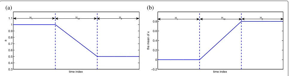
z(n)=a(n)z(n−1)z(n−2)z(n−3)x(n−2)(z(n−3)−1)+x(n−1)
0.3 0.4 0.5 0.6 0.7 0.8 0.9 1 1.1
time index
a
H1 H12 H2
−0.2 0 0.2 0.4 0.6 0.8
time index
the mean of x
H1 H H2
12
(a) (b)
Fig. 1Evolution curves of system parameters:acoefficient a;bmean of x
where the system inputx(n)is a random signal distributed asN(μ, 1)anda(n)is a time-varying system coefficient. The noisy system output is given byy(n) = z(n)+v(n), where the noise v(n) is Gaussian distributed with zero mean and standard deviation 0.1. We change the value of a(n) and the mean ofx(n) with time to simulate a non-stationary scenario: a = 1.0 in the first 1000 samples (segmentH1) and decreases to 0.5 with different change rates (segmentH12) then is fixed toa=0.5 (segmentH2). Similarly, the mean ofx(n)is set at 0 in segmentH1and then linearly increase to 0.8, as shown in Fig. 1. The prob-lem setting for system identification is as follows: the input vector of the kernel filter is
u(n)=[y(n−1),y(n−2),y(n−3),x(n−1),x(n−2)]T and the corresponding design signal is y(n). In this section, both the kernel size and the step size are set at 1.0. The online MSE is calculated based on the mean of the prediction error averaged in a running window of 100 samples.
At first, we compare the performance of QKLMS and QKLMS-MDL when the true system or the input data change slowly, for example, the length of transition area H12 is 1000. The quantization factorγ of QKLMS is set as 0.75 and the window length of QKLMS-MDL is 100
such that both QKLMS and QKLMS-MDL have relatively good compromise between system complexity and accu-racy performance. The simulation results over 200 Monte Carlo runs are shown in Fig. 2. As shown in Fig. 2, the net-work size of QKLMS-MDL is much smaller than QKLMS while their MSE are almost the same. Furthermore, the QKLMS-MDL adjusts the network size adaptively accord-ing to the true system complexity. For example, duraccord-ing the transition of a(n), the system parameters change which increases the signal complexity, but after iteration 2000, the network size decreases gradually signaling that the input signal complexity is reduced. Older centers are dis-carded, and new important centers are added to the center dictionary. On the contrary, QKLMS keeps all existing centers which results in a network size always growing larger.
In order to verify the superiority of QKLMS-MDL, in Table 1, we list the final network sizes of QKLMS and QKLMS-MDL for different transition length condi-tions. The parameter settings are shown in Table 2 where all parameters are selected such that both algorithms yield similar MSE. The final network size of QKLMS-MDL is noticeably smaller than QKLMS. Furthermore, in these different conditions, the final QKLMS-MDL net-work sizes are similar to each other. This fact also testifies
0 500 1000 1500 2000 2500 3000
10−2
10−1
100
time index
MSE
QKLMS QKLMS−MDL
0 500 1000 1500 2000 2500 3000
0 10 20 30 40 50 60 70 80 90
time index
center number
QKLMS QKLMS−MDL
(a) (b)
Table 1The final network size comparison of QKLMS and QKLMS-MDL in a system identification problem
Abrupt change 5001 50001
QKLMS 118.4±4.22 95.08±3.47 124.37±3.52
QKLMS-MDL 12.77±7.55 14.89±9.19 14.23±10.85
All of these results are summarized in the form of “average±standard deviation”
that the network size chosen by QKLMS-MDL is decided by the local complexity of current input data.
4.2 Santa Fe time-series prediction
In this experiment, the chaotic laser time series from the Santa Fe time-series competition, data set A [48] is used [49]. This time series is particularly difficult to pre-dict, due both to its chaotic dynamics and to the fact that only three “intensity collapses” occur in the data set [2], as shown in Fig. 3. After normalizing all data to lie in the range [ 0, 1], we consider the simple one-step pre-diction problem. The previous 40 points u(i) =[x(i − 40),. . .,x(i−1)]T are used as the input vector to predict the current valuex(i)which is the desired response.
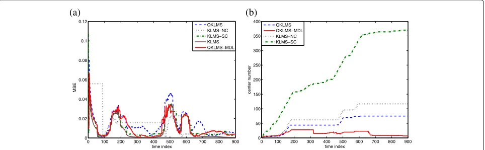
At first, we verify the superiority of QKLMS-MLD ver-sus the QKLMS, the novelty criterion (NC), and surprise criterion (SC), denoted, respectively, as KLMS-NC and KLMS-SC. In the simulation below, the free parameters related to KLMS are set as follows: the Gaussian kernel with kernel width equaling to 0.6 is selected and step size ηis set to 0.9, which were cross-validated in a training set. Performance comparisons between these algorithms are presented in Figs. 4 and 5. In Fig. 4, the parameters of the four sparse algorithms are chosen such that the algorithms yield almost the same maximum network size, while in Fig. 5, the parameters of the sparse algorithms are chosen such that they produce almost the same MSE at the end of adaptation. Table 3 lists the specific parameter settings. Simulation results clearly indicate that the QKLMS-MDL exhibits much better performance, i.e., achieves either a much smaller network size or much smaller MSE than QKLMS, KLMS-NC, and KLMS-SC. Owing to coarse quantization, most of the useful information is discarded by KLMS-NC which results in its learning curve not decreasing after 190 iterations as shown in Fig. 4. Differ-ent from QKLMS, QKLMS-MDL considers the prediction error into quantization and, consequently, has better per-formance. More importantly, the network size of QKLMS-MDL varies. For example, as shown in Fig. 4, the network
Table 2Parameter settings in a channel equalization problem to achieve almost the same final MSE in each condition
Abrupt change 5001 50001
QKLMS γ =0.65 γ=0.7 γ =0.65
QKLMS-MDL Lw=100 Lw=100 Lw=100
size of QKLMS-MDL peaks when the collapse occurs because of local nonstationarity and decreases between time indexes 300 and 400 because the input data com-plexity in this range is well predicted by a lower model. This experiment shows the proposed method has good tracking ability even for data with local nonstationarity.
Then we investigate how the window length affects the system performance. The effect of window length on final MSE and final network size are shown in Figs. 6 and 7, respectively. As shown in Fig. 6, when the window length increases, the final MSE of KLMS-MDL is closer to that of KLMS (for comparison, the final MSE of KLMS also is plotted in the figure). Figure 7 indicates that the increase of the window length results in an increase of the final network size. Fortunately, this growth trend gradually sta-bilizes, such that the network size is limited in a range no matter how long the window length is. In this sense, the window length is also affecting the compromise between system accuracy and network complexity as we can expect from Eqs. 12 and 15, since the window length appears in log form in one of the terms and not in the other.
4.3 Speech signal analysis
Prediction analysis is a widely used technique for the analysis, modeling, and coding of speech signals [1]. A slowly time-varying filter could be used to model the vocal tract, while a white noise sequence (for unvoiced sounds) represents the glottal excitation. Here, we use the kernel adaptive filter to establish a nonlinear pre-diction model for the speech signal. Ideally, for each different phoneme, which represents a window of time series with the same basic statistics, the prediction
0 200 400 600 800 1000
0 0.1 0.2 0.3 0.4 0.5 0.6 0.7 0.8 0.9 1
iteration
0 100 200 300 400 500 600 700 800 900 0
0.02 0.04 0.06 0.08 0.1 0.12
time index
MSE
QKLMS KLMS−NC KLMS−SC KLMS QKLMS−MDL
0 100 200 300 400 500 600 700 800 900
0 5 10 15 20 25 30
time index
center number
QKLMS QKLMS−MDL KLMS−NC KLMS−SC
(a) (b)
Fig. 4Performance comparison in the Santa Fe time-series prediction (the same maximum network size).aConvergence curves in terms of MSE.
bNetwork size evolution curves
model of speech should adjust accordingly to “track” such change. Therefore, we can conjecture to iden-tify the phonetic changes through observing the kernel adaptive filter behavior. For example, when the filter order has local peaks, the phonetics should be chang-ing because the filter observes two different stationary regimes, as demonstrated in Section 4.2. Therefore, such abrupt filter change can be used for phoneme segmenta-tion, which is rather difficult to do even for the human observer.
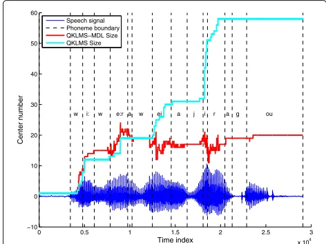
A short whole voiced sentence from a male is used as the source signal. The original voice file can be down-loaded from [50]. To increase the MDL model accuracy when the stationary window is short, this signal is upsam-pled to 16,000 Hz from the original 10,000 Hz. Then QKLMS is applied by the previous 11 samples u(i) = [x(i−11),. . .,x(i− 1)]T. In this section, the Gaussian
kernel withσ =0.3 is selected. The step size is 0.7 accord-ing to the cross-validation test. The quantization factor of QKLMS is set as 0.67 and the window length of
QKLMS-MDL is 50, such that both QKLMS and QKLMS-QKLMS-MDL have relatively similar prediction MSE performance.
Figure 8 shows how the network size of QKLMS-MDL varies with the input speech signal. The phonetic bound-aries are obtained from SPPAS, which is a free audio annotation tool [51, 52]. As show in this plot, the net-work size changes close to the phonetic boundary, like [W] to [e:r] and [j] to [i]. After adapting to the speech (first couple of phonemes), the network size of QKLMS-MDL only changes dramatically during the phoneme transi-tions [e:r], [ei], [i], and [r], because the signal statistics change and the QKLMS-MDL initially increases the pre-diction model due to co-articulation and then decreases it again too much (with an undershoot) until it stabilizes for the remaining of the phoneme. On the other hand, we see that the QKLMS is always increasing size, with the largest rate of increase again during the phoneme transitions. So both respond to the changes in the signal statistics, but QKLMS-MDL preserves a low filter order, with comparable error during the full sentence.
0 100 200 300 400 500 600 700 800 900
0 0.02 0.04 0.06 0.08 0.1 0.12
time index
MSE
QKLMS KLMS−NC KLMS−SC KLMS QKLMS−MDL
0 100 200 300 400 500 600 700 800 900
0 50 100 150 200 250 300 350 400
time index
center number
QKLMS QKLMS−MDL KLMS−NC KLMS−SC
(a) (b)
Fig. 5Performance comparison in the Santa Fe time-series prediction (the same MSE at the final stage).aConvergence curves in terms of MSE.
Table 3Parameter settings for different algorithms in a time-series prediction
Same network size Same final MSE
QKLMS γ =1.97 γ=1.54
QKLMS-MDL Lw=150 Lw=150
KLMS-NC σ1=1.38 σ1=0.85
σ2=0.001 σ2=0.001
KLMS-SC λ=0.005 λ=0.005
T1=90,T2=−0.085 T1=300,T2=−1.6
σ1 the distance threshold,σ2 the error threshold,λthe regularization
parameter,T1the upper threshold of the surprise measure,T2the lower
threshold of the surprise measure
5 Conclusions
This paper proposes for the first time a truly self-organizing adaptive filter where all the filter weight and order are adapted online from the input data. How to choose an efficient kernel model to make a trade-off between computational complexity and system accuracy in nonstationary environments is the ultimate test for an online adaptive algorithm. Based on the popular and powerful MDL principle, a sparsification algorithm for kernel adaptive filters is proposed. Experiments show that the QKLMS-MDL successfully adjusts the network size according to the input data complexity while keep-ing the accuracy in an acceptable range. This property is very useful in nonstationary conditions while other exist-ing sparsification methods keep increasexist-ing the network size. Fewer free parameters and an online model makes QKLMS-MDL practical in real-time applications.
We believe that many applications will benefit from QKLMS-MDL. For example, speech signal processing is an extremely interesting area. Nonstationary behavior is the nature of speech. Furthermore, owing to a sufficient
100 150 200 250 300 350 400 0.004
0.006 0.008 0.01 0.012 0.014 0.016 0.018 0.02 0.022 0.024
window length L
w
finial MSE
MDL−QKLMS KLMS
Fig. 6Effect of the window length on the final MSE in the Santa Fe time-series data
100 150 200 250 300 350 400 4
5 6 7 8 9 10 11 12 13 14
window length Lw
finial network size
Fig. 7Effect of the window length on the final network size in the Santa Fe time-series data
number of samples to quantify short-term stationar-ity, front-end signal processing (acoustic level) based on QKLMS-MDL seems to be a good methodology to improve the quantification of speech recognition because of its fast response. However, this is still a very prelimi-nary paper, and many more results and better arguments for the solutions are required. Although self-organization solves some problems, it also brings new ones in the processing. In fact, as described in Section 3, the QKLMS-MDL algorithm “forgets” in nonstationary conditions the previous learning results and needs to relearn the input-output mapping when the system switches to a new state. First, the filter weights would have to be read and clustered to identify the sequence of phonemes. Sec-ond, the MDL strategy keeps the system model at the simplest structure, but when a previous state appears
0 0.5 1 1.5 2 2.5 3
x 104
−10 0 10 20 30 40 50 60
Time index
Center number
w i: w e:r a w ei a j i r a g ou
Speech signal Phoneme boundary QKLMS−MDL Size QKLMS Size
again, QKLMS-MDL must relearn from scratch because the former centers are removed from the center dictio-nary. This relearning should be avoided, and increas-ingly accurate modeling techniques should be developed. Future work will have to address this aspect of the technique.
Endnotes
1The unit of description length also could benat, which
is calculated by ln rather than log2as we do here. For sim-plification, we use log to present log2in the following part of this paper.
2A translation invariant kernel establishes a
continu-ous mapping from the input space to the feature space. As such, the distance in feature space is monotonically increasing with the distance in the original input space. Therefore, for a translation invariant kernel, the VQ in the original input space also induces a VQ in the feature space.
Acknowledgments
This work was supported by NSF Grant ECCS0856441, NSF of China Grant 61372152, and the 973 Program 2015CB351703 in China.
Authors’ contributions
SZ conceived of the idea and drafted the manuscript. JP, BC, and PZ have contributed in the supervision and guidance of the manuscript. CZ participated in the simulation and experiment. All authors did the research and data collection. All authors read and approved the final manuscript.
Competing interests
The authors declare that they have no competing interests.
Author details
1Department of Electrical and Computer Engineering, University of Florida,
Gainesville, USA.2Institute of Artificial Intelligence and Robotics, Xi’an Jiaotong
University, Xi’an, China.
Received: 20 June 2016 Accepted: 28 September 2016
References
1. W Liu, PP Pokharel, JC Príncipe, The kernel least mean square algorithm. IEEE Trans. Sig. Process.56(2), 543–554 (2008)
2. Y Engel, S Mannor, R Meir, The kernel recursive least-squares algorithm. IEEE Trans. Sig. Process.52(8), 2275–2285 (2004)
3. J Platt, A resource-allocating network for function interpolation. Neural Comput.3(4), 213–225 (1991)
4. P Bouboulis, S Theodoridis, Extension of Wirtinger’s calculus to reproducing kernel Hilbert spaces and the complex kernel LMS. J. IEEE Trans. Sig. Process.59(3), 964–978 (2011)
5. K Slavakis, S Theodoridis, Sliding window generalized kernel affine projection algorithm using projection mappings. EURASIP J. Adv. Sig. Process.1, 1–16 (2008)
6. C Richard, JCM Bermudez, P Honeine, Online prediction of time series data with kernels. IEEE Trans. Sig. Process.57(3), 1058–1066 (2009) 7. W Liu, Il Park, JC Príncipe, An information theoretic approach of designing
sparse kernel adaptive filters. IEEE Trans. Neural Netw.20(12), 1950–1961 (2009)
8. B Chen, S Zhao, P Zhu, JC Príncipe, Quantized kernel least mean square algorithm. IEEE Trans. Neural Netw. Learn. Syst.23(1), 22–32 (2012)
9. B Chen, S Zhao, P Zhu, JC Príncipe, Quantized kernel recursive least squares algorithm. IEEE Trans. Neural Netw. Learn. Syst.24(9), 1484–1491 (2013)
10. SV Vaerenbergh, J Via, I Santamana, A sliding-window kernel RLS algorithm and its application to nonlinear channel identification. IEEE Int. Conf. Acoust. Speech Sig. Process, 789–792 (2006)
11. SV Vaerenbergh, J Via, I Santamana, Nonlinear system identification using a new sliding-window kernel RLS algorithm. J. Commun.2(3), 1–8 (2007) 12. SV Vaerenbergh, I Santamana, W Liu, JC Príncipe, Fixed-budget kernel
recursive least-squares. IEEE Int. Conf. Acoust. Speech Sig. Process, 1882–1885 (2010)
13. M Lázaro-Gredilla, SV Vaerenbergh, I Santamana, A Bayesian approach to tracking with kernel recursive least-squares. IEEE Int. Work. Mach. Learn. Sig. Process. (MLSP), 1–6 (2011)
14. S Zhao, B Chen, P Zhu, JC Príncipe, Fixed budget quantized kernel least-mean-square algorithm. Sig. Process.93(9), 2759–2770 (2013) 15. D Rzepka, in2012 IEEE 17th Conference on Emerging Technologies & Factory
Automation (ETFA). Fixed-budget kernel least mean squares, (Krakow, 2012), pp. 1–4
16. K Nishikawa, Y Ogawa, F Albu, inSignal and Information Processing Association Annual Summit and Conference (APSIPA). Fixed order implementation of kernel RLS-DCD adaptive filters, (Asia-Pacific, 2013), pp. 1–6
17. K Slavakis, P Bouboulis, S Theodoridis, Online learning in reproducing kernel Hilbert spaces. Sig. Process. Theory Mach. Learn.1, 883–987 (2013) 18. W Gao, J Chen, C Richard, J Huang, Online dictionary learning for kernel
LMS. IEEE Trans. Sig. Process.62(11), 2765–2777 (2014)
19. J Rissanen, Modeling by shortest data description. Sig. Process.14(5), 465–471 (1978)
20. M Li, PMB Vitányi,An introduction to Kolmogorov complexity and its applications. (Publisher, Springer-Verlag, New York Inc, 2008) 21. H Akaike, A new look at the statistical model identification. IEEE Trans.
Autom. Control.19(2), 716–723 (1974)
22. G Schwarz, Estimating the dimension of a model. Ann. Stat.6(2), 461–464 (1978)
23. A Barron, J Rissanen, B Yu, The minimum description length principle in coding and modeling. IEEE Trans. Inf. Theory.44(6), 2743–2760 (1998) 24. J Rissanen, Universal coding, information, prediction, and estimation. IEEE
Trans. Inf. Theory.30(4), 629–636 (1984)
25. J Rissanen, MDL denoising. IEEE Trans. Inf. Theory.46(7), 2537–2543 (2000) 26. L Xu, Bayesian Ying Yang learning (II): a new mechanism for model
selection and regularization. Intell. Technol. Inf. Anal, 661–706 (2004) 27. Z Yi, M Small, Minimum description length criterion for modeling of
chaotic attractors with multilayer perceptron networks. IEEE Trans. Circ. Syst. I: Regular Pap.53(3), 722–732 (2006)
28. T Nakamura, K Judd, AI Mees, M Small, A comparative study of information criteria for model selection. Int. J. Bifurcation Chaos Appl. Sci. Eng.16(8) (2153)
29. T Cover, J Thomas,Elements of information theory. (Wiley, 1991) 30. M Hansen, B Yu, Minimum description length model selection criteria for
generalized linear models. Stat. Sci. A Festschrift for Terry Speed.40, 145–163 (2003)
31. K Shinoda, T Watanabe, MDL-based context-dependent subword modeling for speech recognition. Acoust. Sci. Technol.21(2), 79–86 (2000) 32. AA Ramos, The minimum description length principle and model
selection in spectropolarimetry. Astrophys. J.646(2), 1445–1451 (2006) 33. RS Zemel,A minimum description length framework for unsupervised
learning, Dissertation. (University of Toronto, 1993) 34. AWF Edwards,Likelihood, (Cambridge Univ Pr, 1984)
35. M Small, CK Tse, Minimum description length neural networks for time series prediction. Astrophys. J.66(6), 066701 (2002)
36. A Ning, H Lau, Y Zhao, TT Wong, Fulfillment of retailer demand by using the MDL-optimal neural network prediction and decision policy. IEEE Trans. Ind. Inform.5(4), 495–506 (2009)
37. JS Wang, YL Hsu, An MDL-based Hammerstein recurrent neural network for control applications. Neurocomputing.74(1), 315–327 (2010) 38. YI Molkov, DN Mukhin, EM Loskutov, AM Feigin, GA Fidelin, Using the
minimum description length principle for global reconstruction of dynamic systems from noisy time series. Phys. Rev. E.80(4), 046207 (2009) 39. A Leonardis, H Bischof, An efficient MDL-based construction of RBF
40. H Bischof, A Leonardis, A Selb, MDL principle for robust vector quantisation. Pattern Anal. Appl.2(1), 59–72 (1999)
41. T Rakthanmanon, EJ Keogh, S Lonardi, S Evans, MDL-based time series clustering. Knowl. Inf. Syst., 1–29 (2012)
42. H Bischof, A Leonardis, in15th International Conference on Pattern Recognition. Fuzzy c-means in an MDL-framework, (Barcelona, 2000), pp. 740–743
43. I Jonye, LB Holder, DJ Cook, MDL-based context-free graph grammar induction and applications. Int. J. Artif. Intell. Tools.13(1), 65–80 (2004) 44. S Papadimitriou, J Sun, C Faloutsos, P Yu, Hierarchical, parameter-free
community discovery. Mach. Learn. Knowl. Discov. Databases., 170–187 (2008)
45. E Parzen, On estimation of a probability density function and mode. Ann. Math. Stat.33(3), 1065–1076 (1962)
46. AM Mood, FA Graybill, DC Boes,Introduction to the Theory of Statistics. (McGraw-Hill, USA, 1974)
47. SA Geer,Applications of empirical process theory. (The Press Syndicate of the University of Cambridge, Cambridge, 2000)
48. The Santa Fe time series competition data. http://www-psych.stanford. edu/~andreas/Time-Series/SantaFe.html, Accessed June 2016 49. AS Weigend, NA Gershenfeld,Time series prediction: forecasting the future
and understanding the past. (Westview Press, 1994)
50. Sound files obtained from system simulations. http://www.cnel.ufl.edu/~ pravin/Page_7.htm, Accessed June 2016
51. B Bigi, inThe eighth international conference on Language Resources and Evaluation. SPPAS: a tool for the phonetic segmentations of Speech, (Istanbul, 2012), pp. 1748–1755
52. SPPAS: automatic annotation of speech. http://www.sppas.org, Accessed June 2016
Submit your manuscript to a
journal and benefi t from:
7Convenient online submission
7Rigorous peer review
7Immediate publication on acceptance
7Open access: articles freely available online
7High visibility within the fi eld
7Retaining the copyright to your article