Regularized orthogonal least squares algorithm for constructing radial basis function networks

(1)

This article was downloaded by:[University of Southampton] On: 13 September 2007

Access Details: [subscription number 773565843] Publisher: Taylor & Francis

Informa Ltd Registered in England and Wales Registered Number: 1072954 Registered office: Mortimer House, 37-41 Mortimer Street, London W1T 3JH, UK

International Journal of Control

Publication details, including instructions for authors and subscription information:

http://www.informaworld.com/smpp/title~content=t713393989

Regularized orthogonal least squares algorithm for

constructing radial basis function networks

S. Chena; E. S. Chngb; K. Alkadhimia

a_{Department of Electrical and Electronic Engineering, University of Portsmouth,} Portsmouth, U.K.

b_{Department of Electrical Engineering, University of Edinburgh, Edinburgh, U.K.} Online Publication Date: 01 July 1996

To cite this Article: Chen, S., Chng, E. S. and Alkadhimi, K. (1996) 'Regularized orthogonal least squares algorithm for constructing radial basis function networks', International Journal of Control, 64:5, 829 - 837

To link to this article: DOI: 10.1080/00207179608921659 URL:http://dx.doi.org/10.1080/00207179608921659

PLEASE SCROLL DOWN FOR ARTICLE

Full terms and conditions of use:http://www.informaworld.com/terms-and-conditions-of-access.pdf

This article maybe used for research, teaching and private study purposes. Any substantial or systematic reproduction, re-distribution, re-selling, loan or sub-licensing, systematic supply or distribution in any form to anyone is expressly forbidden.

(2)

Downloaded By: [University of Southampton] At: 18:04 13 September 2007

Regularized orthogonal least squares algorithm for constructing radial

basis function networks

S. C H E N t , E. S. CHNGS and K. A L K A D H I M I t

The paper presents a regularized orthogonal least squares learning algorithm for radial basis function networks. The proposed algorithm combines the advantages of both the orthogonal forward regression and regularization methods to provide an efficient and powerful procedure for constructing parsimonious network models that generalize well. Examples of nonlinear modelling and prediction are used to demonstrate better generalization performance of this regularized orthogonal least squares algorithm over the unregularized one.

1. Introduction

For practical purposes, it is desired to construct a small neural network. Apart from some obvious advantages, small models often generalize better. The orthogonal least squares (OLS) algorithm (Chen et al. 1991) is a n efficient procedure for learning a parsimonious radial basis function (RBF) network. A simple mechanism can be built into the algorithm to avoid automatically any ill-conditioning of learning problems. For B-splines neural networks (Brown and Harris 1994), a learning procedure called ASMOD (Kavli 1993) has been developed for constructing parsimonious models. The parsimonious principle alone, however, is not entirely immune to overfitting. If data are highly noisy, small models constructed may still fit into noise. A technique for overcoming overfitting is regularization. This technique is usually applied to large full- size neural networks (Poggio and Girosi 1990, Bishop 1991).

Some researchers have combined regularization techniques with the parsimonious principle. For example, Barron and Xiao (1991) proposed a first-order regularized stepwise selection of subset regression models. A recent study (Orr 1993) has applied both the forward regression and zero-order regularization techniques to construct parsimonious R B F networks with improved generalization properties. The zero-order regularization is a technique equivalent to simple weight-decaying in gradient descent methods for multilayer perceptron neutral networks (Hertz et al. 1991). It is also known as the ridge regression in the statistical literature (Hoerl and Kennard 1970). Although these regularized subset selection algorithms are capable of choosing a small model with improved generalization properties, they require considerably more computation than the OLS algorithm.

This paper combines the zero-order regularization with the OLS algorithm to derive a regularized OLS (ROLS) algorithm for R B F networks. This new forward selection algorithm is capable of constructing small R B F networks which generalize

Received 18 December 1995. Revised 19 July 1995.

t

Department of Electrical and Electronic Engineering, University of Portsmouth, Anglesea Building, Portsmouth PO1 3DJ, U.K.

$Department of Electrical Engineering, University of Edinburgh, King's Buildings, Edinburgh EH9 3JL, U.K.

(3)

well. Furthermore, it has a similar computational requirement to that of the O L S algorithm and is, therefore, computationally very efficient. For the notational simplicity, RBF networks with a single output node are considered in this paper. However, the results can readily be applied to multi-output R B F networks (Chen et (11.

1992). The effectiveness of the ROLS algorithm is demonstrated using a modelling and prediction application.

2. Formulation of linear regression model

Before describing the ROLS algorithm, we formulate the R B F network as a linear regression model. The R B F network with m inputs, n, hidden nodes and a scalar output is defined by

where x = [x,

...

xmlT is the input vector, 0, are the weights, c, = [c,,,

...

c,,,lT are the R B F centres, 11.11 denotes the euclidean norm and #(.) is known a s the nonlinearity of hidden nodes. Two examples of #(.) are the thin-plate-spline function d(r) = r210g(r) and the gaussian function #(r) = exp(-r2/pZ), where p

>

0 is a width parameter.

Assume that we have a training set of N samples {d(r),x(t)},N_,, where d(t) is the target or desired network output corresponding to the network input vector ~ ( 1 ) . Assume for the time being that we use every x(t) a s a centre, that is, c, = x(& for

1

<

i

<

N. Then the actual network outputs are

The model (2) may be referred to as the 'full' network model. By introducing the notation #,(t) = &\lx(r)-c,ll), we can express the desired output d(t) as

where e(t) is the error between d(t) and f,(x(t)). By defining

we can collect (3) for I

<

t

<

N together as

(4)

Regularized orthogonal least squares algorithm 831

1 $ i < N, can be referred to as regressors. In practice, it is often necessary to

select a smaller subset of n, centres or regressors from the full model (2).

3. The regularized OLS algorithm

The error criterion used in deriving the OLS algorithm (Chen et al. 1991) is the total squared error eTe. The least squares criterion in certain circumstances is prone to overfitting. To prevent overfitting, regularization techniques can be applied. In the study of Orr (1993), a regularized forward selection (RFS) algorithm was derived by considering the zero-order regularized error criterion

where

A

2 0 is the regularization parameter. The RFS algorithm selects one centre from the full model (9) at a time. Each selection is chosen to decrease maximally the regularized squared error (10). A drawback of this algorithm is that it cannot utilize an orthogonalization scheme and therefore requires considerably more computation than the OLS algorithm.

We can actually combine the zero-order regularization with the OLS algorithm to form an efficient procedure for subset selection. Let an orthogonal decomposition of the regression matrix @ be

where

and

W=[w,

...

w,]

with orthogonal columns that satisfy

w:w,=O, i f i S j

The full model (9) can be rewritten as

d = Wg+e

The orthogonal weight vectorg = [ g ,

...

g,lT and the original weight vector 8 satisfy the triangular system

(5)

832 S. Chen et al.

The key to derive a computationally efficient ROLS scheme is to consider the following zero-order regularized error criterion

It is obvious that the criterion (17) is similar to the criterion (lo) due to the relationship (16). In fact, the term IgTg penalizes large g,, which is equivalent to penalizing large 0,.

After some simple calculations, it can be shown that the regularized error criterion (1 7) can be expressed as

Normalizing (18) by d T d yields

Similar to the case of the OLS algorithm (Chen er al. 1991), we can define the

regularized error reduction ratio due to w, as

[rerr],

=

(wT w,

+

I)g,2/dTd (20)

Based on this ratio, significant regressors can be selected in a forward-regression procedure exactly as in the case of the OLS algorithm (Chen et al. 1991). The selection

is terminated at the nHth stage when

"H

I - [rerr],

<

c

is satisfied, where 0

<

1 is a chosen tolerance. This produces a subset network containing n, significant regressors. The ROLS algorithm based on the modified Gram-Schmidt scheme is given in the Appendix.

It should be emphasized that the solution found by the ROLS algorithm is identical to that found by the RFS algorithm of Orr (1993). Both algorithms perform a subset model selection based on the forward search technique. The ROLS algorithm, however, requires considerably less computation than the RFS by exploiting some orthogonal properties. The forward selection is a suboptimal method and does not guarantee to find the optimal solution. To find the optimal nH-term subset model from an N-term full model, it is required to calculate the performance of all possible nH-term subset models and to choose the best one. This is computationally prohibitive even for a modest N and thus impractical. A subset model found using the forward selection technique is generally good enough for many practical applications.

4. Choice of regularization parameter

(6)

Regularized orthogonal least squares algorithm 833

Kennard 1970, Golub et al. 1979). A previous study using the second-order regularization (Bishop 1991) has suggested that the performance of the RBF network may be fairly insensitive to the precise value of l .

An elegant approach to the selection of the regularization parameter is to adopt a Bayesian interpretation and to calculate the best value of regularization parameter using the evidence procedure (Mackay 1992). Applying this Bayesian approach to the ROLS algorithm results in the following iterative procedure for estimating

I.

Given an initial guess of 1, the algorithm constructs a network model. This in turn allows an uptading of 1 by the formula

where

is the number of good parameter measurements (Mackay 1992). After a few iterations, an appropriate

R

value can be found.

5. Examples

In the first example, the RBF network with a gaussian basis function and a width p = 0.2 is used to approximate the scalar function

Ax) = sin (2rrx), 0

<

x $

1 (24)

One hundred training data were generated fromAx)+e, where x was taken from the uniform distribution in (0 1) and the noise > , e had a aaussian distribution with zero

-

mean and standard deviation 0.4. A separated test data set was also generated for

x = 0,0.01,

.. .

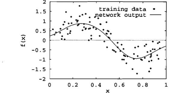
,0.99,1.00. The training data and the functionflx) are plotted in Fig. 1. The training data set is highly ill-conditioned. The ROLS algorithm selected 15 centres from the training set.

Figure 2 depicts the mean square error (MSE) as a function of log,,(l) for both the training and testing data sets. The optimal value of 1 for this example is approximately 1.0. However, for a large range of l values, the MSE over the testing set is quite flat, indicating that the performance of the ROLS algorithm is fairly insensitive to the precise value of l in this large region. Figure 3 shows the network mapping constructed by the ROLS algorithm with 1 = 1.0. As a comparison, the network mapping constructed by the OLS algorithm is given in Fig. 4, where overfitting can be clearly seen.

(7)

[image:7.611.186.440.80.264.2] [image:7.611.192.437.293.450.2] [image:7.611.154.437.479.634.2]

S. Chen et al.

Figure I . Noisy training data (points) and underlying function (curve).

0.6 0.55

::

0.5

0.45

a 0.4

h

a

Oi3;

(0

0.25 0.2 0.15 0.1

-8 -6 -4 -2 0 2 4 log10 (lambda)

Figure 2. Mean square error as a function of the regularization parameter.

training data

.

.**. eetwork output -

1

(8)

Regularized orthogonal least squares algorithm

t r a i n i n g data -

[image:8.617.168.418.91.268.2] [image:8.617.170.416.297.452.2]

.

. o o , ; l e t w o r k o u t p u t -

Figure 4. Network mapping constructed by the orthogonal least squares algorithm.

ROLS OLS

-

r

0.05

0 5 10 15 2 0

p r e d i c t i o n step

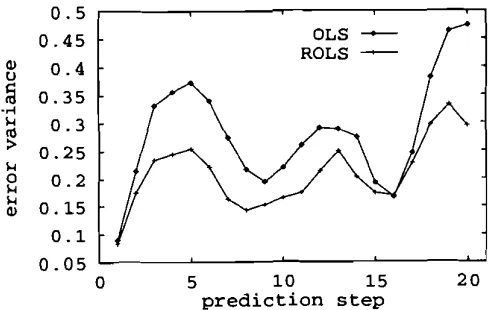
Figure 5. Normalized variances of multi-step prediction errors for the sunspot time series over years 192 1-1955.

other nonlinear models fitted to the time series (Weigend et al. 1990, Chen and Billings 1989).

As a comparison, the ROLS algorithm was used to construct a RBF network of 25

centres based on the same full network model with

I

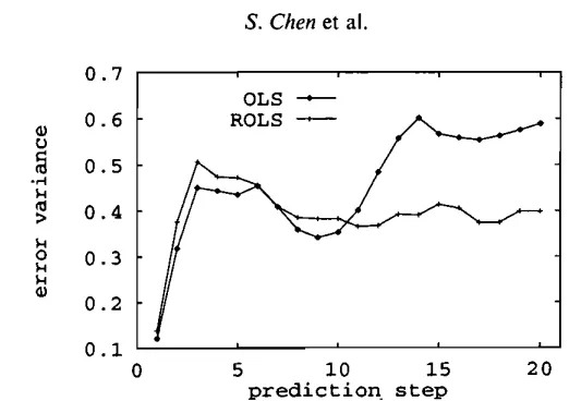
= lo7. Figure 5 compares the predictive performance of this model over the period 1921-1955 with that of the network constructed using the OLS algorithm. Predictive accuracies of the two network models obtained using the ROLS and OLS algorithms respectively over the period 1921-1979 are plotted in Fig. 6. The results shown in Figs 5 and 6 clearly demonstrate that the ROLS algorithm has better generalization properties.

(9)

S. Chen et al.

OLS

-

ROLS

-

0 5 10 15 20

p r e d i c t i o n . step

Figure 6. Normalized variances of multi-step prediction errors for the sunspot time series over years 1921-1979.

6. Conclusions

A very efficient learning algorithm for radial basis function networks has been derived by combining the orthogonal-least-squares forward selection and the zero- order regularization technique. This algorithm is capable of constructing parsimonious radial basis function networks which generalize well under severely noisy conditions. Although the method has been presented in the context of radial basis function networks, it can actually be applied to all the nonlinear models that have a linear-in-the-parameters structure, such as the fuzzy basis function network and the Volterra series model.

Appendix

The modified Gram-Schmidt orthogonal procedure calculates the A matrix row by row and orthogonalizes @ as follows: at the kth stage make the columns k + l

<

j

<

N , orthogonal to the kth column and repeat the operation for

1

<

k

<

N- 1. Specifically, denoting

@?)

= Gj, 1 $ j $ N , then

w* =

@y'

a k , j = w ~ @ y - l ) / ( w ~ ~ k ) , k + l < j < N k = 1 , 2

,...,

N-l

I

(A 1)

@y-l)-ak,Jw,,k+l < j < N

The last stage of the procedure is simply w, = @f-". The elements o f g are computed by transforming d''' = d i n a similar way

where

I

3 0 is the regularization parameter.

This orthogonalization scheme can be used to derive a simple and efficient algorithm for selecting subset models. First introduce the definition of @'*-I) as

W-l) = [wl

. . .

Wk-l @Lk-l'

. .

.

@ y ] _(A₃₎ If some of the columns @:-I),

.

. .

,

@:-I) in @'k-l) have been interchanged, this will still [image:9.612.178.439.82.266.2]

(10)

Regularized orthogonal least squares algorithm

S t e p 1 . F o r k

<

j

<

N, compute

g;j) = (@y-l))Tdk-l)/((@y-l))T @?-I)

+ A )

[rerrlf' = (gi'))Z((@y-l))T @?-I)

+

12)/ffd

S t e p 2. Find

I

[rerr], = [rerrlij*) = max {[rerr]L1), k

<

j

<

N)

Then t h e j,th column o f @"-" is interchanged with the kth column o f @ ( k - ' ) ,

a n d the j,th column o f A is interchanged u p t o the (k- l)th r o w with the kth

column o f A . This effectively selects the j,th candidate a s the k t h regressor in

the subset model.

Step 3 . Perform the orthogonalization a s indicated in (A 1) t o derive the kth row o f A

a n d t o transform @'k-l) into @'"'. d"-" is then updated into d'*) in the way

shown in (A 2).

T h e selection is terminated a t the n,th stage when the criterion (21) is satisfied a n d this produces a subset model containing n , significant regressors.

REFERENCES

BARRON, A. R., and XIAO, X., 1991, Discussion of multivariate adaptive regression splines.

Annals of Statistics, 19, 67-82.

BISHOP, C., 1991, Improving the generalization properties of radial basis function neural networks. Neural Computation, 3, 579-588.

BROWN, M., and HARRIS, C. J., 1994, Neurofuzzy Adaptive Modelling and Control (Hemel

Hempsted, U.K.: Prentice Hall).

CHEN, S., 1994, Radial basis functions for signal prediction and system modelling. Journal of

Applied Science and Computations, 1 .

CHEN, S., and BILLINGS, S. A,, 1989, Modelling and analysis of non-linear time series.

International Journal of Control, 50, 2 15 1-2 17 1.

CHEN, S., COWAN, C. F. N., and GRANT, P. M., 1991, Orthogonal least squares learning

algorithm for radial basis function networks. IEEE Transactions on Neural Networks, 2, 302-309.

CHEN, S., GRANT, P. M., and COWAN, C. F. N., 1992, Orthogonal least squares algorithm for

training multi-output radial basis function networks. Proceedings of the Institution of

Electrical Engineers Pt F , 139, 378-384.

GOLUB, G. H., HEATH, M., and WAHBA, G., 1979, Generalized cross-validation as a method for

choosing a good ridge parameter. Technornetrics, 1, 21 5-223.

HERTZ, J., KROUGH, A,, and PALMER, R., 1991, Introduction to the TheoryofNeural Computation

(Redwood City, California, U.S.A.: Addison-Wesley).

HOERL, A. E., and KENNARD, R. W., 1970, Ridge regression: biased estimation for non-

orthogonal problems. Technometrics, 12, 5S67.

KAVLI, T., 1993, ASMOD: an algorithm for adaptive spline modelling of observation data.

International Journal of Control, 58, 947-968.

MACKAY, D. J. C., 1992, Bayesian interpolation. Neural Computation, 4, 415-447.

ORR, M. J. L., 1993, Regularised centre recruitment in radial basis function networks. Research

Report, No. 59, Centre for Cognitive Science, University of Edinburgh, U.K.

Pocclo, T., and GIROSI, F., 1990, Networks for approximation and learning. Proceedings of the

lnstitution of Electrical and Electronics Engineers, 78, 1481-1497.

TONG, H., 1983, Threshold Models in Non-linear Time Series Analysis (New York: Springer- Verlag).

WEIGEND, A. S., HUBERMAN, B. A., and RUMELHART, D. E., 1990, Predicting the future: a

http://www.informaworld.com/smpp/title~content=t713393989

http://dx.doi.org/10.1080/00207179608921659

http://www.informaworld.com/terms-and-conditions-of-access.pdf