Mobility in wireless sensor networks : advantages, limitations and effects

(1)

Mobility in Wireless Sensor

Networks: Advantages, Limitations

and Effects

AMU

THE AUSTRALIAN NATIONAL UNIVERSITY

A thesis submitted for the Degree of

Doctor of Philosophy of

The AustraUan National University

Oday Jerew

July 2011

(2)

{ umm

A

(3)

Declaration

The contents of this thesis are the results of original research and have not been submitted for a high degree to any other university or institution.

Much of the work in this thesis has been published or has been submitted for publication.

Conference Papers

• Oday D. Jerew, Haley M. Jones, and Kim L. Blackmore, On the Minimum Number of Neighbours for Good Routing Performance in MANETs, In Proc. of International Conference on Mobile Ad Hoc and Sensor Systems

(MASS09), IEEE, pages 12-15, October, 2009.

• Oday Jerew and Weifa Liang, Prolonging Network Lifetime Through the Use of Mobile Base Station in Wireless Sensor Networks. In Proc. of International Conference on Advances of Mobile Computing and Multimedia (MoMM), ACM, pages 170-178, December, 2009.

Journal papers

• Oday Jerew, Kim Blackmore and Weifa Liang, Mobile Base Station and Clustering to Maximize Network Lifetime in Wireless Sensor Networks. IEEE Transaction on Wireless Communications (to be submitted).

• Oday Jerew and Kim Blackmore, Multipath Routing Scheme For Mobile Relays in Wireless Sensor Networks. IEEE Transaction on Wireless Communications (to be submitted).

Oday Jerew and Kim Blackmore, Estimation of Hop Count in Multihop Paths in Sparse and Dense Ad Hoc and Sensor Networks. IEEE Transaction on Vehicular Technology (to be submitted).

c

o . ^ .

(4)

(5)

Ill

Acknowledgements

Without the support of the many faces in my hfe, this work would not have been possible. I would like to acknowledge and thank each of the followings:

• First of all, I would like to show my deep appreciation for my advisor, Dr. Kim Blackmore, for her guidance, support, encouragements, and patience. Her deep insight brought me a lot of ideas that were invaluable for all of my work.

• I would like to thank the amazing Dr.Tony Flynn, for his helpfulness, support and patience, not to mention his sense of humour and optimism. This thesis would certainly not been possible without his support.

• I would like to thanks Dr. Haley Jones and Dr. Weifa Liang for their helpful ideas, insight, feedback and general rock-solid reliability as a supervisor. • I would like to thank the Iraqi Ministry of Higher Education and Scientific

Research to provide me with the opportunity and financial to come to ANU and conduct research work.

• My thanks to the Department of Engineering and Information Technology in ANU for their supportive and the use of their facilities in the production of this thesis.

• Last, but definitely not least, I would like to thank my parents: mum and dad and my wife for their moral support, love and for always being there when I need them.

(6)

(7)

Abstract

The primary aim of this thesis is to study the benefits and hmitations of using a mobile base station for data gathering in wireless sensor networks. The case of a single mobile base station and mobile relays are considered.

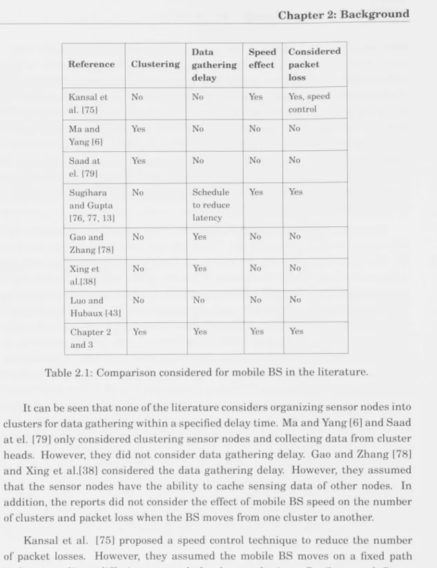
A cluster-based algorithm to determine the trajectory of a mobile base station for data gathering within a specified delay time is presented. The proposed algorithm aims for an equal number of sensors in each cluster in order to achieve load balance among the cluster heads. It is shown that there is a tradeoff between data-gathering delay and balancing energy consumption among sensor nodes. An analytical solution to the problem is provided in terms of the speed of the mobile base station. Simulation is performed to evaluate the performance of the proposed algorithm against the static case and to evaluate the distribution of energy consumption among the cluster heads. It is demonstrated that the use of clustering with a mobile base station can improve the network lifetime and that the proposed algorithm balances energy consumption among cluster heads. The effect of the base station velocity on the number of packet losses is studied and highlights the limitation of using a mobile base station for a large-scale network.

We consider a scenario where a number of mobile relays roam through the sensing field and have limited energy resources that cannot reach each other directly. A routing scheme based on the multipath protocol is proposed, and explores how the number of paths and spread of neighbour nodes used by the mobile relays to communicate affects the network overhead. We introduce the idea of allowing the source mobile relay to cache multiple routes to the destination through its neighbour nodes in order to provide redundant paths to destination. An analytical model of network overhead is developed and verified by simulation. It is shown that the desirable number of routes is dependent on the velocity of the mobile relays. In most cases the network overhead is minimized when the source mobile relay caches six paths via appropriately distributed neighbours at the destination.

A new technique for estimating routing-path hop count is also proposed. An analytical model is provided to estimate the hop count between source-destination pairs in a wireless network with an arbitrary node degree when the network nodes are uniformly distributed in the sensing field. The proposed model is a significant improvement over existing models, which do not correctly address the low-node density situation.

(8)

(9)

Vll

Abbreviations

AODV BFS BS CDF CEDAR CGSR DSDV DSR GPS LCA LEACH MAHSN MR PC PDA PDF RREP RREQ RCH RS TORA UAV VCH v s WLAN WRP WSN ZRP Cov{p, r) Area(.) [•] r-i E{.} [•J max{.} min{.} Pr

Ad Hoc On-Demand Distance Vector Breadth First Search

Base Station

Cumulative Distribution Function

Core Extraction Distributed Ad Hoc Routing Cluster-head Gateway Switch Routing Destination-Sequenced Distance-Vector Dynamic Source Routing

Global Positioning System Linked Cluster Algorithm

Low-Energy Adaptive Clustering Hierarchy Mobile Ad Hoc Sensor Network

Mobile Relay Personal Computer

Personal Digital Assistants Probability Density Function Route Reply

Route Request Real Cluster Head Real Segment

Temporally Ordered Routing Algorithm Unmanned Aerial Vehicles

Virtual Cluster Head Virtual Segment

Wireless Local Area Network Wireless Routing Protocol Wireless Sensor Network Zone Routing Protocol

A circular region centred at position p with radius r

Area Average Operator Ceiling Operator Expectation Operator Floor Operator Maximum Operator Minimum Operator Probability

(10)

(11)

List of Figures

1.1 Sensor networks [1] 8

1.2 A two-layer hierarchical sensor network [2] 10

1.3 Mobile sensors (MRs) are used to provide connection between

discon-nected network [3] 11

1.4 Using mobile sensors (MRs) to extend the lifetime of the bottleneck

nodes [4] 12

2.1 Network lifetime using direct communication and

minimum-transmission energy routing [5] 21

2.2 Sensors that remain alive are indicated by circles and sensors that are dead are indicated by dots. The BS located at 100 m from the closest sensor node, x = 0, y = - 1 0 0 rn. (a) For direct routing, (b) For

minimum-transmission energy routing [5] 21

3.1 An example of clustering procedure, PQ is the centroid location of sensing field. Pi and Pz are the locations of two boundary sensor nodes, Py G P\P2, and AK is the cluster area, (a) Area (PQ: Pi,P2)>

AK. (b) Area (PQ. PJ , P z H AK 34

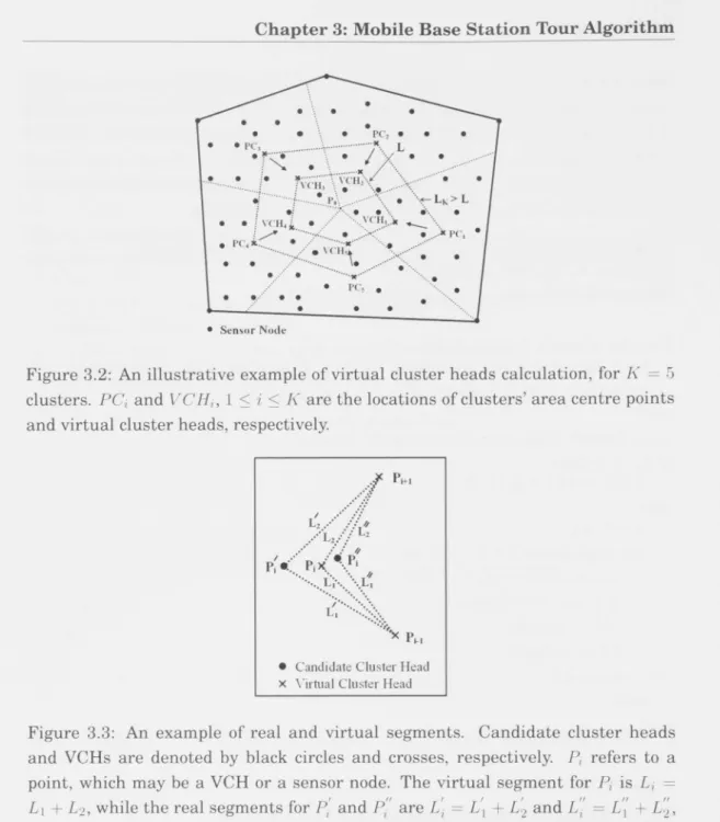
3.2 An illustrative example of virtual cluster heads calculation, for K = 5 clusters. P Q and VCH^, \ <i < K are the locations of clusters' area

centre points and virtual cluster heads, respectively. 38

3.3 An example of real and virtual segments. Candidate cluster heads and VCHs are denoted by black circles and crosses, respectively. Pj refers to a point, which may be a VCH or a sensor node. The virtual segment for Pj is L^ = Li + L2, while the real segments for P^ and

(14)

LIST OF FIGURES

3.4 An execution example of finding real cluster heads, K = 5 clusters, (a) Finding two candidate cluster heads for each cluster, one with RS^ > VS^ and the other with RS^ < VSi, I < i < K. (b) After the execution of Phase I, sensor nodes 04 and 05 are selected as real cluster heads since they are closest to VCHi, VCH5 and B.S4 < VS4, RS5 < VS5, respectively, (c) Then, sensor node 61 is selected as real cluster head since it is closest to VCHi and L2 < Lk- (d) After the execution of Phase II, sensor nodes 02 and 03 are initially selected as real cluster heads, then 03 is changed with 63 as real cluster head since it is closest to VCHj, and L4 < Lk, 62 is not selected as a real cluster head since the corresponding BS tour length is greater than

LK 42 4.1 The mobile BS data gathering scenario 47

4.2 The effect of the number of clusters on the CDF of the percentage of number of packet losses, from (4.5) when r = 100 rn, Vm ^ 2 ni/s, n = 3500, Trq = 10 ms and Tp = 200 ms, where m meter, s second and rns millimeter. For these settings, the approximate minimum

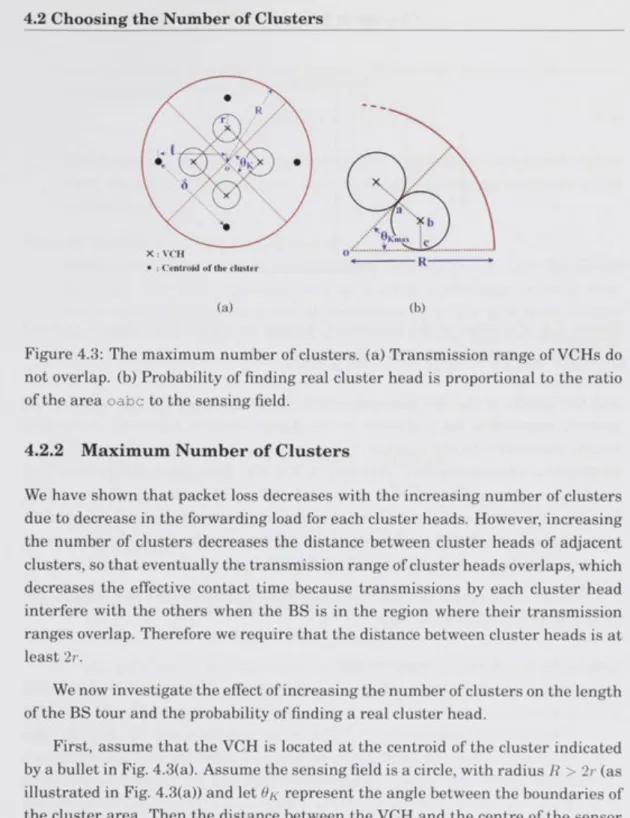
number of clusters, Kmin, is eight from (4.2) 48 4.3 The maximum number of clusters, (a) Transmission range of VCHs

do not overlap. (b) Probability of finding real cluster head is

proportional to the ratio of the area o a b c to the sensing field 49 4.4 The effect of the number of clusters on the BS tour when r = 1 and

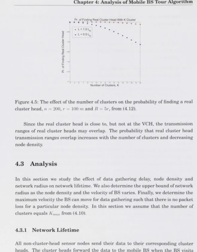
R = 5r. Kmax is calculated from (4.9) 50 4.5 The effect of the number of clusters on the probability of finding a

real cluster head, n = 200, r = 100 m and R = 5r, from (4.12) 52 4.6 The effect of network radius on the CDF of number of packet losses,

from (4.4) and (4.5), at relaxed delay requirement, from (4.9). We have r = 100 rn, = 2 rn/s, Trq = 10 rns, Tp = 200 ms and d = 15, so Us = 499. The approximate upper bound of network radius R <

6.98 fcm from (4.16) 55

4.7 The effect of the BS velocity on the approximate minimum number of clusters, from (4.2), when Trq = 10 rns, Tp = 200 rns and d = 15. The

approximate maximum number of clusters from (4.10), when R = 5r. 56 4.8 Network lifetime as it varies with network radius, for our algorithm,

SenCar algorithm [6], and the maximum lifetime for the same numbers of clusters. The maximum network lifetime is calculated from (4.13), which assumes all clusters have the same number of nodes. 58 4.9 The energy consumption for neighbouring sensor nodes of a cluster

head for our algorithm and SenCar algorithm [6] as the network

(15)

LIST OF FIGURES

4.10 Network lifetime as it varies with node degree, for static and mobile BSs with different K. The maximum network lifetime is calculated from (4.13), which assumes all clusters have the same number of nodes. 60 4.11 The minimum and maximum energy consumption differences among

the cluster heads as the node degree is varied 60 4.12 The energy consumption for neighbouring sensor nodes of a cluster

head as the node degree is varied, for various numbers of clusters. . 61 4.13 The maximum number of hops as it varies with the node degree, for

static and mobile BSs 61 4.14 The percentage of network packet loss as the number of network

sensor nodes are varied, for varies number of clusters 62 4.15 The minimum cluster head neighbouring sensor nodes energy

con-sumption as the node degree is varied, for various data gathering

delay 63 4.16 The maximum number of hops as it varies with the node degree, for

static and mobile BSs 64

5.1 Comparison of next hop zone proposed in the literature, rii represents the source or intermediate node and rij represents the destination or next-hop node, (a) Hou at al. in [7]. (b) Kleinrock and Silvester in [8]

and Kuo and Liao in [9] (c) Wang at el. in [10] 66 5.2 Hop count as it varies with different node degree and distance

between the source and destination 68 5.3 Simulation results of 25 randomly selected paths between source, S,

and destination, D, nodes. Nodes are deployed with uniform distribu-tion in the sensing field, (30r x SOr ), the source and destinadistribu-tion nodes placed at (7.5r, 15r) and (15.5r, 15r), respectively. LO = 8r and R = 1

unit length, (a) d = 2. (b) ci = 5. (c) d = 8. (d) d = 16 69 5.4 Simulation results of the next hop of 100 paths between source, S, and

destination, D, nodes. Nodes are deployed with uniform distribution in the sensing field, (3()r X 30r), the source and destination nodes are placed at (7.5r, 15r) and (15.5r, 15r), respectively LO = 8r and r = 1

unit length, (a) d = 2. (b) d = 5. (c) rf = 8. (d) d = 16 71 5.5 Effective relaying region between n, and Uj. (a) A path with a single

intermediate hop exists as there is an effective neighbour in Ai region, (b) A path exists as there is an effective neighbour in A2

region for both n^ and Uj 72 5.6 The PDF of the angle between the next hop and destination nodes at

different node degrees, = 8r 73 5.7 The PDF of normahzed hop progress (r = 1) at different node degrees,

(16)

LIST OF FIGURES

5.8 An example illustrates the distance relationship between source node, Hs, neighbour node, nj and destination node, rid- rii is neighbour to Us at distance do,i and angle B^. Ls d is the distance between Ug and Ud, Od is the position angle of n^. L^.i is the remaining distance to destination after selecting rii as the next hop. Lsd - Lr,i is the hop

progress 75 5.9 An example illustrates the order of neighbour nodes according to its

distance to destination for d = 4 76 5.10 Expected hop progress, from (5.4) as it varies with the order of

neighbour (distance to destination), for different node degree when

r = l 77 5.11 The probability of selecting the nearest neighbour node to

destina-tion, from (5.5) as it varies with node degree at 2 < d < 6 78 5.12 The probability of selecting the neighbour node, from (5.6) as it varies

with the order of neighbour node for different node degree at 2 < d < 6. 79 5.13 Hop progress from (5.8), as it varies with node degree when LSD =

Br-and r = 1 80 5.14 Connectivity probability as it varies with different node degrees,

from (5.9) 81 5.15 Hop progress as it varies with node degree, theoretical results from

(5.8) and Wang et al. in [10]. Simulation results are depicted by

markers while theoretical results are depicted by lines 82 5.16 The hop count as it varies with node degree, theoretical results from

(5.11) and Wang et al. in [10]. Simulation results are depicted by

markers while theoretical results are depicted by lines 83

6.1 An example illustrates how the source augments the routes to be through the neighbour node that is closest to the direction of

movement of the source 89 6.2 An example illustrates the selection of cr = 4 neighbour nodes at the

destination MR from a total of d = 9 physical neighbours. The total variation of the chosen neighbours from the ideal of 6'-separation is

e error = 01 + 9-2 + 63 90

6.3 An example of two neighbour nodes, rii and n2, at angles 0\ and 62 and distance do,i and do,2, respectively. The MR moves in a straight line in direction 0m- Grey dots indicate MR location when the links

to rii and 712, respectively, fail 93

6.4 Normalized link residual time as it varies with the number of neighbour nodes and initial distance, between 0 and r from (6.3). . . 93

(17)

LIST OF FIGURES

6.5 Circles have radius, r, centred on the nearest neighbour, n^, which is

located at distance do,i from the MR. The MR moves in the direction

of angle S^. The direction of movement is denoted by a dotted line. . . 94 6.6 The PDF of link residual time between MR and its neighbour from

from (B.l), (B.3) and (B.5) in Appendix B. The MR moves in random

direction with v velocity. 95 6.7 Example illustrates that the source and destination MRs move in

random directions. The ns cached multiple routes to through different neighbour nodes. The direction of movement is denoted by

a dotted arrow line 95 6.8 An example illustrates source MR cached routes to destination MR

through appropriately distributed neighbour nodes of the destina-tion, rii, n2 and n^. Nodes 712 and 713 are two adjacent neighbours to

MR at angles S2 and 63, respectively, from the direction of movement. 98 6.9 The CDF of the link residual time, for our scenario, where ns moves

between two neighbours from (6.16), (6.18) and (6.20). The angle between the direction of movement and neighbours varies from tt/G

to 7r/2 and the node moves at velocity vo = O.lr 100 6.10 The PDF of the cache residual time, for randomly selected neighbours

from (6.12) and our routing scheme from (6.24) when the number of

paths equals to 5 and 8 and v = vs = vp 101

6.11 Overhead as it varies with source and destination MRs velocities, for passive and active multipath, (6.32) and (6.36), respectively.

LSD = and d = 6. Simulation results are depicted by markers

while theoretical results are depicted by lines 107 6.12 Overhead in a dense network as it varies with source and destination

MRs velocities, for randomly selected paths and our multipath

routing scheme, (6.36) and (6.37), respectively. Lso = ^r and d = 20.

Simulation results are depicted by markers while theoretical results

are depicted by lines 109 6.13 Overhead comparison in a dense network as it varies with source

and destination MRs velocities, our multipath routing scheme, for randomly selected paths and the Braided scheme [11]. Lso = ^r and

(18)

(19)

List of Tables

2.1 Comparison considered for mobile BS in the literature 24

2.2 Comparison of using MRs 28 4.1 Definitions of the main symbols used throughout this chapter. . . . . 46

4.2 The approximate minimum number of clusters as it varies with node degree, from (4.2). The approximate Kmax = 10, from (4.10) at

(20)

LIST OF TABLES

(21)

Chapter

1 Introduction

1.1 Thesis Motivation

The research described in this thesis has been largely motivated by the perceived need for understanding of the effect of the use of mobility in Wireless Sensor Networks (WSNs) on network performance. The potential benefits and limitations of using single and multiple mobile entities for data gathering has only recently been fully recognised [12][13].

Data gathering in WSNs is one of the most frequent and fundamental operations, and requires the sensor nodes to monitor the sensing field for as long as possible. As sensor nodes have limited energy resources and are powered by small batteries, energy consumption is a critical issue in the design of WSNs that effect network lifetime.

Some WSNs use mobility to prolong network lifetime by allowing a mobile base station (BS) to roam a sensing field and gather data from sensor nodes through a short transmission range. The energy consumption of each sensor node is then reduced, since fewer relays are needed for the sensor node to relay its data packet to the BS. As the speed of mobile BS is very slow compared with the speed of data packets which travel in multi-hop forwarding, the increased latency of data gathering when employing mobile BS presents a major performance bottleneck. Thus, the time a mobile BS takes to tour a large sensing field may not meet the stringent delay requirements inherent in some mission-critical, real-time applications. Therefore, planing the trajectory and determining the speed of mobile BS need to be considered in order to achieve the delay requirements.

Planning the moving tour of a mobile BS is a critical issue in the maximization of network lifetime and meeting data-gathering delay requirements. In order to maximize network lifetime, a mobile BS collects data using single-hop

(22)

commu-Chapter 1: Introduction nication, which requires a long time since it has to visit each sensor node. On the other hand, using multi-hop communication to reduce data-gathering time increases sensor-node power consumption and thus shortens network lifetime.

Data-gathering time could also be decreased by increasing the speed of the mobile BS. However, the contact time between the mobile BS and sensor nodes is decreased and thus increases the probability of packet losses. In addition, the network lifetime and number of packet losses increase when the network scale is expanded. Thus the use of a mobile BS is not sufficient to achieve the required network performance of a large scale network.

The moving of sensor nodes has been introduced in the literature in order to achieve requirements such as improve converge and connectivity or improve network lifetime by moving to a new location to help bottleneck sensors by inheriting sensing, transmission and receiving responsibilities. Several algorithms for planning the trajectory of the mobile BS have been proposed to prolong network lifetime, which do not analyse the limitations when the network scale is expanded and investigate the effect of BS velocity on packet losses.

Multiple mobile entities, which we refer to as mobile relays (MRs) are proposed to roam the sensing field and buffer sensing data to be forwarded to the BS. MRs are used to improve network lifetime as the network scale is expanded. However, little attention is paid to the routing between MRs. Most of the literature assumes that MRs can interact with each other directly in order to send sensing data to the BS, where this can be achieved either by restricting the mobility area of MRs which adds more constraint to trajectory planning or by assuming the MRs have unlimited energy resources to reach each other and the BS. Thus, there is a need for further investigation into the effect of the mobility of MRs on routing performance as the mobility inevitably incurs additional overhead in data communication protocols, whose overhead can potentially offset the benefit brought by mobility.

The mobility of sensor nodes in the sensing field forms mobile ad hoc networks. Therefore, in the following section, we introduce the main properties of ad hoc networks, mobile ad hoc networks and then sensor networks.

1.2 Ad Hoc Networks

A wireless ad hoc network is a collection of nodes with no pre-established infras-tructure. Each node has a wireless communication capability to communicate with others. Since there is no central entity in ad hoc networks the nodes must

(23)

1.3 Mobile Ad Hoc Networks

participate in order to organise themselves into a network. Ad hoc networks show a distinct departure from traditional infrastructure wireless networks such as cellular networks and WLANs, in that there is no need for a central access point or BS. In ad hoc networks, nodes that are within each other's transmission range can communicate directly and are responsible to discover each other. These nodes are often energy constrained, that is, batteries are the main energy resource with a great diversity in their capabilities. Therefore, the transmission range of nodes is limited. Intermediate nodes work as routers in order to relay data packets between nodes that are not lie within each transmission range. That is, data packets need to be delivered over a path involving multiple nodes (multi-hops).

1.2.1 Wireless Signal Propagation Model

In wireless ad hoc networks, electromagnetic radio waves are used for commu-nication. When radio waves travel through media which contains many objects, they experience several propagation mechanisms such as reflection, diffraction and scattering. The wireless channel (transmission medium) is susceptible to a variety of transmission impediments such as path loss, interference, and blockage. These factors restrict the range, data rate, and the reliability of the wireless transmission and places fundamental limitations on the performance of wireless communication systems [14], Therefore the transmission range of nodes varies in time and space. This i referred to as the physical layer in the Open Systems Interconnection (OSI) reference model (a standard model used to describe computer network architecture).

The data link layer of the OSI model is responsible for ensuring reliable frame communication by detecting and possibly correcting errors that may occur in the physical layer. The network layer then uses these frames to generate packets and is concerned with routing the packets to their destination [15]. In this thesis we ignore physical layer effects, and instead deal with the network layer by considering the routing path of data packets such that the power consumption of wireless nodes is minimized. Therefore, we assume in Chapters 3, 5 and 6 signal attenuation is due only to path loss related to distance transmitted.

1.3 Mobile Ad Hoc Networks

Nodes in ad hoc network could be cellular phones, personal digital assistants (PDAs), pocket PCs and laptops. These nodes are mobile and have to join or leave the network when they move arbitrarily, this resulting in rapid and

(24)

Chapter 1: Introduction unpredictable topology changes. In this energy-constrained, dynamic, multi-hop environment, nodes need to organise themselves dynamically in order to provide the necessary network functionality in the absence of fixed infrastructure or central administration. Thus a mechanism for path identification and maintenance is needed.

Due to node mobility and variation in transmission-range power, mobile ad hoc networks experience a high level of topology variability. All the nodes must participate to provide network functions, such as data forwarding and routing activities, in order to self-organize network topology. Node mobility strongly influences the performance of the network. Therefore, an efficient routing protocol is needed to improve network performance such as route delay, loop free routing, control overhead, scalability and power conservation.

1.3.1 Routing Protocols For Mobile Ad Hoc Networks

Ad hoc wireless network-routing protocols can be classified into three major types based on the routing information update mechanism as follows [15]:

1. Proactive (table-driven) routing protocols: Every node in this type of protocol maintains the network topology information in the form of routing tables by continuously evaluating the routes within the networks, so that when a packet needs to be forwarded, the route is already known and can be immediately used. This has the advantage that when a route is needed, the delay before packets can be sent is very small. However, it needs some time to converge to a steady state which can cause problems when the topology is changing frequently. Typical proactive routing protocols include: Destination-Sequenced Distance-Vector Routing (DSDV), Cluster-head Gate-way Switch Routing (CGSR) and the Wireless Routing Protocol (WRP). 2. Reactive (On-demand) routing protocols: A node in this reactive routing

protocol obtains the necessary path to destination when it is required, by using a type of global-search procedure. Thus, these protocols do not exchange routing information periodically. This form of routing may suffer a long delay since a route to destination needs to be acquired before sending a data packet. Dynamic Source Routing (DSR), Ad Hoc On-Demand Distance Vector (AODV) and Temporally Ordered Routing Algorithm (TORA) are examples of on-demand routing protocols.

Any on-demand routing protocol must utilise some type of routing cache in order to avoid the need to rediscover each routing decision for each individual packet. One of the critical factors in an on-demand routing protocol is the

(25)

1.3 Mobile Ad Hoc Networks

setting of the cache timeout value, since the route cache may rely on links between nodes that are no longer within wireless transmission range of each other. A large route cache timeout causes some stale information to be employed degrading network performance rather than improving it. On the other hand, small route cache timeout cause a number of valid routes to be removed before they expire and hence are an inefficient use of cache information.

3. Hybrid routing protocols: This type combines the features of proactive and reactive routing protocols. Often nodes in a network are divided into routing zones based on particular geographic regions. Routing within the same zone is implemented based on proactive routing, while reactive routing is used for routing among nodes that belong to different zones. The Linked Cluster Algorithm (LCA), Core Extraction Distributed Ad Hoc Routing (CEDAR) and Zone Routing Protocol (ZRP) are examples of this type of routing protocol.

1.3.2 E f f e c t of M o b i l i t y o n R o u t i n g P e r f o r m a n c e

Mobility in ad hoc networks is one of the most challenging in the design of routing protocols, since nodes can roam sensing fields independently of each other at varying velocities. In general, most of the literature that studies the effect of mobility in ad hoc networks shows that network performance is degraded due to link failures, that cause a significant number of routing packets to discover new paths, leading to increased network congestion and transmission latency.

Intensive research has been done on the effect of mobility on routing protocols and compares their performance using different routing-protocol metrics. Metrics used to evaluate the performance of routing protocols include [16, 17, 18, 19]:

• Throughput: Throughput measures the effectiveness of the network in deliv-ering data packets. That is, the amount of data packets that is successfully transferred over a period of time.

• Packet delivery ratio: The ratio of the number of packets received to the number of packets sent.

Routing overhead: The number of routing control packets requested when a data packet is successfully dehvered to the destination.

End-to-end delay: The average time difference between the time a packet is sent from the source and the time it is successfully received by the destination.

(26)

Chapter 1: Introduction The on-demand routing protocols such as DSR and AODV perform better than the proactive, such as DSDV at high mobility rates, while DSDV perform quite well at low mobility rates [17][20], since the proactive routing protocols update the routing table whenever the network topology changes. Thus, proactive protocols are not suitable for mobile ad hoc networks in which the network topology changes frequently [21], In addition, the performance also differs for on-demand routing protocols, for example, using the packet dehvery ratio and end-to-end delay as performance metrics, DSR outperforms AODV in less demanding situations, while AODV outperforms DSR in heavy traffic load and high mobility, while, the routing overhead of DSR is lesser than that of AODV [18][20]. This is because many of their routing mechanics are different. In particular, DSR uses source routing, whereas AODV uses table driven routing framework and destination sequence numbers.

Exploring the manner in which mobility affects network communication can help the design of an efficient routing protocol. Several routing-protocol schemes have been designed that rely on identification of stable links in the networks by assuming nodes perform online measurements [22][23]. The stable links are then preferentially used for routing.

Investigating the effect of mobility using mobility metrics is necessary to measure the reliability of individual paths and discover long-lived routes. Routing protocols based on mobility metric [24, 25, 26] have shown there is an improvement in network performance such as packet delivery ratio and network overhead when mobility prediction metric is used. The prediction metric is used to predict the duration of time that two nodes remain connected.

Link residual time is a mobility metric that is used to measure the time during which two nodes are within transmission range of each other. The time until the route breaks, path residual time, can then be measured, where the reliability of a path depends on the availability of all links constituting the path. In this research, path residual time is used to decide when a path is broken and a new route request needs to be initiated.

1.3.3 Effect of Node Density

Node density, which is the number of nodes in a unit area, is another factor that effects network performance. As the network nodes are deployed randomly without any wired infrastructure and communicate via multi-hop wireless links, node density effects the connectivity of the nodes in the network. Network connectivity can be increased by increasing the number of nodes (for a fixed network area). However, increasing the number of nodes tends to reduce the effective bandwidth available for each node due to increased competition for bandwidth. In addition,

(27)

1.4 Wireless Sensor Networks

it increases the traffic load, contention and packet collision between neighbour nodes. On the other hand, when the number of nodes is small, the network may not be fully connected and therefore some nodes cannot send packets to certain destinations [27], Increasing the transmission power of a node can achieve a higher transmission range and therefore nodes can reach more nodes via a direct links. In contrast, a node that uses a very low transmission power may become isolated without any link to other nodes. Thus, the network connectivity depends on both node density and their transmission range [28],

Connectivity is often associated with the number of neighbours (node degree). Many investigations have been conducted for the evaluation of the minimum number of neighbours needed for full connectivity in a wireless network [8, 29, 30, 31, 32] . It was first proposed by Kleinrock and Silvester in [8] that six was the 'magic number', i.e., on average every node should connect itself to its six nearest neighbours, and various papers since then have argued for magic numbers between five and eight [33, 7, 34, 35]. In this research, we use node degree as a measure of node density (rather than the number of nodes in a unit area), since it reflects the number of nodes that can be accessed using the maximum transmission range.

The node degree has a significate effect of the number of hops between the source and destination nodes. As we will demonstrate in Chapter 5, the number of hops is approximately proportional to the separation distance for very low or very high node degree, but significantly greater for node degree close to the 'magic number' values. In general, a path with a high number of hops increases the end-to-end delay and wastes the bandwidth.

1.4 Wireless Sensor Networks

Sensor networks are a special category of ad hoc wireless networks that include sensor nodes which are tiny devices that have the capability of sensing physical parameters, processing the data gathered, and communicating over the network to send data to the monitoring station (sink or BS). A sensor network is a collection of a large number of sensor nodes that are deployed in a particular region. Fig. 1.1 illustrates a traditional homogeneous wireless sensor network with flat architecture, where all nodes are equipped with identical battery capacity and hardware complexity, except for the sink node as the gateway to communicate with end users across the Internet [1].

Some of the domains of application for sensor networks are military, health care, home security, and environmental monitoring. Some of the issues that distinguish the sensor networks category of ad hoc wireless networks are as

(28)

Chapter 1: Introduction

Sink

Task manager node

User

Sensor field Sensor nodes

Figure 1.1: Sensor networks [1], follows:

• Mobility of nodes: Nodes in wireless sensor networks are not assumed to be fully mobile, enabling all or a subset of nodes to provide stationary sensing abilities.

• Size of the network (scalability): The network size of sensor networks is much larger than that in ad hoc networks.

• Node density: The node density in sensor networks is larger than in ad hoc networks, which offer a small number of hops between the source and destination in sensor networks.

• Power constraints: Nodes are considered to be highly energy constrained as battery reserves are not easily replenished.

• Data sink, In general, nodes in wireless sensor networks send data packets (sensing data) to a sink, while in ad hoc networks any two nodes could be the source and destination of data packets.

The topology of WSNs is variable due to both mobility of a subset of nodes and node failures (due to energy issues). The goal of WSNs is to reduce the energy consumption of sensor node, in order to prolong its lifetime. Protocols must be designed which enable power conservation at the expense of degradation in throughput and delay characteristics.

A flat network architecture for WSNs leads to several challenges in terms of routing design, energy conservation and network management. Therefore, a hierarchical sensor network architecture is introduced, in the following section.

(29)

1.4 Wireless Sensor Networks

1.4.1 Hierarchical Sensor Network Architecture

Energy efficiency and scalability are the greatest challenges in the design of sensor networks. Therefore, hierarchical sensor network architecture is often employed in which sensors are organized into clusters with a cluster head in each cluster Cluster heads collect sensing data and make routing and scheduling decisions.

Hierarchical sensor networks can be classified into two broad types; homoge-neous and heterogehomoge-neous sensor networks [36]. In homogehomoge-neous networks all the sensor nodes are identical in terms of battery energy and hardware complexity. Some of the nodes are selected to serve as cluster heads. However, cluster heads consume more energy than other sensor nodes and as a result the cluster head fails before other nodes. Rotating the role of cluster head randomly and periodically over network nodes can help to balance energy consumption among cluster heads and hence increase the overall cost of the entire sensor network [37], However, dynamically selected cluster heads can incur a high overhead due to frequent exchange of control packets among sensor nodes [2].

On the other hand, in a heterogeneous sensor network, one or more different types of nodes in addition to sensor nodes with different energy resources and functionality are used. The basic idea behind that is more complex hardware and extra battery energy can be embedded in cluster head nodes and can help to reduce the hardware cost of the rest of the resource limited basic sensor nodes. For instance, a two-tier hierarchical sensor network is shown in Fig. 1.2 where two types of sensor nodes are deployed in the sensing area, basic sensor nodes with limited communication capability that are mainly used for sensing the environment and sensor nodes with more powerful transceivers and batteries that act as cluster heads. The cluster head organizes basic sensor nodes into clusters, gathers sensing data and then forwards these to the BS. Clustered sensor networks can be classified as single-hop and multi-hop. A single-hop network is one in which sensor nodes use single-hop communication to reach the cluster head. In a multi-hop network nodes use multi-hop communication to forward sensing data to reach the cluster head. In both cases, the cluster heads use single-hop to reach the BS.

1.4.2 Mobility in Wireless Sensor Networks

Recent research [12][13] shows that significant energy saving can be achieved in wireless sensor networks by using mobile devices capable of carrying data mechanically. In this approach, a small number of mobile devices roam about sensing fields and collect data from sensors. As a result, significant network

(30)

Chapter 1: Introduction

Outside Observer

y / — ^ ^ ^ Cluster Head Layer

Figure 1.2: A two-layer hierarchical sensor network [2],

energy saving can be achieved by reducing or completely avoiding costly multi-hop wireless transmissions.

Mobility in WSNs can be achieved by using vehicles or people carrying sensors. The energy consumption of mobile devices is less constrained as they can replenish their energy supplies because of their mobility. However, the primary disadvantage of this approach is increased latency. For instance, the typical speed of several practical mobile device systems is approximately 0.1 — 1 m/s [38]. Thus, it takes more t h a n 16 min for a mobile device to take a tour of length 1 Km to g a t h e r sensing data, which may not meet the delay requirements of some data-intensive applications.

In some applications like disaster m a n a g e m e n t it is more efficient to use vehicles since the environmental conditions are harsh. The mobile device could also be carried using aerial and remotely piloted vehicles [39], For instance, a n u m b e r of u n m a n n e d aerial vehicles (UAVs) such as helicopters can co-operate with ground sensor nodes for data gathering in mission-critical application. Generally, the mobility of BS can be classified into three types according to the mobility p a t t e r n of the entity upon which the BS is mounted as follows:

1. Random Mobility: This can be achieved for example when the BS is mounted on h u m a n s and animals [40], in this case the probability of the BS collecting all sensing data is low since the BS opportunistically visits sensor nodes. 2. Predictable Mobihty: In this case the BS is mounted on an entity t h a t moves

on a fixed track or path t h a t cannot control its direction or speed, but which moves at a regular time, for example a BS mounted on a bus or train. Thus, the sensor nodes can predicate when the BS may move around to send their data [41][42].

3. Controlled Mobility: When the BS is mounted on a robot or UAV plane, then the direction and speed of the BS can be controlled. Several algorithms are

(31)

1.4 Wireless Sensor Networks

mobile sensors

Figure 1.3: Mobile sensors (MRs) are used to provide connection between disconnected network [3].

proposed to find the trajectory of the BS in order to achieve some requirement such as maximise network hfetime and data-gathering delay using single and multi-hop relays.

Most literature considers the mobility of WSNs to be predictable or con-trolled [2, 41, 43, 44, 45, 4] to achieve network performance requirements (some literature considers random mobility to improve network lifetime), which differs from mobile ad hoc networks in which nodes are assumed to move arbitrarily which degrades the network performance by link failures.

In this research we classify mobile entities used in WSNs into two categories: mobile BS and MR. Mobile BS has unlimited energy sources with high buffering and processing capabilities. MRs may be similar to static sensors (limited transmission range and storage) with movement capability or have higher storage capability to buffer and carry sensing data to be sent to the BS.

In general, mobility in WSNs is used to:

• Improve network coverage: Sensor nodes are usually randomly deployed in the sensing field by scattering from aircraft or by robots [46] which cannot be guaranteed to cover the whole area. Coverage requires that each location in the sensing field be monitored by sensors. An MR relocates its position in order to cover the required sensing field.

• Improve network connectivity: MRs relocate to provide a connection path between several non-connected subnetworks [3][47] as shown in Fig. 1.3. • Carrying data from isolated sensors: MRs with store-carry-forward capability

can travel between isolated sensors to collect sensing data and then forward it to a BS [48, 47, 49, 50, 51, 52].

• Improve network lifetime: Mobile BS and MRs can be used to improve network hfetime. Where MRs can move to a new location to help bottleneck

(32)

Chapter 1: Introduction Mobile 0 ^ Sensor A Sensor B Sensor A Mobile 6 ^ Sensor B Phase 1 Pliase 2

Figure 1.4: Using mobile sensors (MRs) to extend the lifetime of the bottleneck nodes [4],

sensors by inheriting sensing, transmission and receiving responsibilities. For example, Wang et al. [4] assume the network shown in Fig. 1.4. The whole network is composed of two components that are connected via sensors A and B. Thus, these two sensors are the bottleneck nodes since they have to forward all network traffic between the two components. An MR can inherit the responsibility of sensor A and B at some time and thus the network lifetime is improved. A mobile BS and MRs can roam a sensing field (connected/disconnected) and gather data from sensor nodes through a short transmission range. The energy consumption of each sensor node is then reduced, since fewer relays are needed for the sensor node to relay its data packet to the BS. In order to maximize network lifetime, mobile BS and MR can collect data using single-hop communication, however, that increases data-gathering delay since the mobile BS and MRs have to visit the transmission range of each sensor node. On the other hand, using multi-hop communication for data gathering decreases data-gathering delay and decreases network lifetime. Therefore, path planning of a mobile BS and MRs is a critical issue in maximization of network lifetime and to meeting data-gathering delay requirements.

1.5 Contributions

Our contribution in this research can be divided into two parts:

• We consider data gathering in a mobile BS environment, subject to a specified tour delay-time constraint on the mobile BS, by adopting a clustering-based approach. To reduce the energy consumption of a cluster head to forward

(33)

1.6 Thesis Overview

sensing data, the mobile BS roams the sensing field and visits only the cluster heads to gather sensing data. Therefore, the distribution of the cluster heads in the entire network affects the load balance among the sensor nodes and hence the network lifetime.

We propose a heuristic algorithm for finding a trajectory of the mobile BS consisting of cluster heads which meet the following criteria: (i) the energy consumption among the sensor nodes within any cluster is balanced in order to prolong network lifetime; and (ii) the total traversal time of the mobile BS on the trajectory is bounded by a given value. The proposed algorithm significantly increases the network lifetime.

We then conduct a detailed analysis to the proposed algorithm. We analyti-cally study the upper and lower bounds on the number of clusters such that there is no packet lost due to moving too fast through a cluster or interference between cluster heads. Statistical methods are used to determine the probability of finding cluster heads and of losing packets as the BS moves from one cluster to another

We propose a routing scheme to provide interaction between MRs and BS, where MRs are used for data gathering from sensor nodes that are moving at relatively lower speed than MRs. An analytical model is needed to study the effect of mobility of MRs on routing performance as the mobility inevitably incurs additional overhead in data-communication protocols, where that overhead can potentially offset the benefit brought by mobility.

We consider a multipath routing extension of DSR, where separate routes via each neighbour are stored in the cache. In this case the number of neighbouring nodes, and hence paths, effects the network overhead. We develop an analytical model, verified by simulation, for the network as a function of the MR speed, distance to the BS, and node density. The results reveal that the proposed routing scheme can significantly reduce routing overhead, however, the number of cached routes stored should be limited to six to prevent overhead blowout when the MR moves quickly.

1.6 Thesis Overview

In Chapter 2 we present the background and related work. We introduce the techniques used to reduce the energy consumption and evaluate the network lifetime in static sensor networks. We highlight the use of mobility to reduce energy consumption and prolong network lifetime. We define the mobile entities in WSN

(34)

Chapter 1: Introduction as mobile BS and MRs. We survey the related literature that consider finding moving trajectory for a mobile BS and the interaction among MRs.

In Chapter 3 we introduce the idea of reducing the energy consumption of sensor nodes using mobile BS for data gathering. We consider data gathering in a mobile BS environment, subject to a specified tour delay time constraint on the mobile BS, by adopting a clustering-based approach.

In Chapter 4 we provide analysis of the proposed algorithm. We show the benefit and limitation when a mobile BS is used for data gathering. We analytically study the upper and lower bounds on the number of clusters such that there is no packet lost due to moving of BS too fast through a cluster or interference between cluster heads. We use statistical methods to determine the probability of finding cluster heads and of losing packets as the BS moves from one cluster to another.

In Chapter 5 we propose an analytical model to estimate the hop count between source-destination pairs when the network nodes are uniformly distributed in the sensing field. This model is used for calculating the expected overhead in Chapter 4. To calculate the number of hops in the path, we determine a distribution describing the remaining distance from next-hop node to destination. We calculate the probability of selecting each of the neighbour nodes. The expected number of hops needed to cover the remaining distance is calculated by obtaining the expected progress towards the destination. The hop count model is verified by simulation.

In Chapter 6 we propose a routing scheme for MRs interaction. Multipath routing is consider to provide redundant paths to destination. The link residual time between MR and its neighbours is analysed. We explore how the number of paths and spread of neighbour nodes used by the source MR to reach the destination affects the network overhead. The speed of MRs is evaluated in order to minimize the network overhead due to mobility. An analytical model is developed and verified by simulation.

Finally, in Chapter 7, we present an overview of the results presented and suggestions for future work.

(35)

Chapter

2 Background

Energy consumption is a crucial consideration for sensor networks and their applications as sensor nodes are commonly battery-driven. Once sensor nodes are deployed, it is challenging and sometimes even impossible to change batteries. Hence, the network lifetime becomes a critical concern in the design of WSNs.

The lifetime of a sensor network can be defined in different ways, according to the effect of losing sensor nodes on the functionality of the whole network, which depends on the sensor network application [53]. For instance, network lifetime could be defined as the time until the first node depletes its battery. On the other hand, a network could be considered to be alive as long as a given percentage of the sensors has enough energy to operate. In this case, the network lifetime is defined as the time for which a given percentage of the region is covered by live sensors. In this research we define network lifetime as the time the first node fails, which is the definition most frequently found in the literature.

Data gathering in sensor networks can be divided into two types according to the specific needs of the applications, these are time-driven and event-driven. In a time-driven scenario all sensors send data periodically to the sink. As opposed to this, in the event-driven case sensors start communicating with the sink only if sensing an event, i.e., a situation that is worth reporting according to the requirements of the application. In this research we address the time-driven scenario, and provide energy-efficient solutions for homogeneous networks, with sensors having constant and equal amounts of data to send in all parts of the sensing field. In the following section, we list some techniques that are used to reduce energy consumption in ad hoc and sensor networks.

(36)

Chapter 2: Background

2.1 Techniques to Reduce Energy Consumption

Nodes in wireless ad hoc and sensor networks consume energy in sensing, processing, transmission and reception. Communication functions expend most of the node energy. In the following we present different techniques to reduce energy consumption of ad hoc and sensor nodes related to communication.

2.1.1 Energy-efficient Routing Schemes

Sensed data in ad hoc and sensor networks are usually sent to its destination using multiple-hop communication. The level of transmission power is assumed to be adjusted to the minimum level required to ensure the intended receiver is within the transmission range. The selection of the next hop in the routing path effects the energy consumption of nodes, since the power level will be adjusted depending on the choice of the next hop node [54]. The aim of this technique is to maximize network lifetime by selecting:

• a path to minimize the total energy consumed to reach the destination, which minimizes the energy consumption per unit flow; and/or

• the path with nodes with the highest residual energy.

The network lifetime can also be prolonged by using a multipath routing protocol with a view to providing load balancing among network nodes. A multipath routing protocol can choose to divert traffic through alternative paths to ease the burden of the congested link. Moreover, multipath routing can provide fault tolerance by having redundant information routed to the destination via alternative paths. This reduces the probability that communication is disrupted in the case of link failure which minimizes the control overhead required to discover a new route.

The selection of paths is one of the challenging issues in multipath routing that effect the network performance and has been studied extensively in the literature. The most commonly used criterion is the disjointness of paths, which classifies the paths in terms of shared resources as follows [55]:

Node-disjoint: There are no common nodes in the paths except the source and destination nodes.

(37)

2.1 Techniques to Reduce Energy Consumption

• Partially disjoint: There are common links and intermediate nodes among paths.

Selecting paths with minimum common nodes and links reduces the proba-bility that a link-failure effects multiple paths. However, selecting paths with disjoint-nodes is difficult in some situations and the discovered paths may have more hops than the shortest hop path, which is not energy efficient [11]. Therefore, in Chapter 6 we propose a routing scheme to find multipath routes between the source and destination. The routes are selected via different neighbour nodes for the source and destination in order to reduce the probability of path failure.

2.1.2 Data Aggregation

Data aggregation is a common technique used in sensor networks. In most WSN applications, sensor nodes are used to detect environmental events and send sensing data to a BS. In event-driven applications, it is required to detect a particular environmental phenomenon (for example to detect when a temperature exceeds 60 degrees at specified time intervals). During that time interval all sensors send their data packets towards the BS. Thus, there are a large number of data packets needing to be sent to the BS, with some of them redundant since some sensor nodes are used to detect the same environment events.

The base idea in data aggregation techniques is to reduce packet complexity at the intermediate nodes and minimize energy consumption of the sensor nodes by taking advantage of correlations among sensing data [56]. Correlation refers to the data redundancy between two sensor packets due to the overlap of sensing activi-ties. The nature of correlation differs with the type of applications considered [57].

Clustering can be used to reduce the amount of data required to be sent to a BS. The sensing field is divided into small clusters, a cluster head being responsible for aggregating and relaying to the BS the data gathered from the sensors of its clusters [58][59]. One of the most cited clustering approaches is LEACH (Low-Energy Adaptive Clustering Hierarchy), a self-organising, adaptive protocol where the nodes organise themselves into clusters, with one node acting as the cluster head. The cluster head aggregates the sensing data and then transmits the compressed data to the BS [5]. This can achieve a reduction in energy consumption, as data aggregation is much cheaper than communication.

Once the cluster-head has all the data from the nodes in its cluster, the cluster-head node aggregates the data and then transmits the compressed data to the BS. In Chapter 3 we consider data gathering by adopting a cluster-based approach. Sensor nodes send their data to the cluster heads. The cluster heads

(38)

Chapter 2; Background forward sensing data to the BS without data aggregation. Thus, the cluster heads consume more energy than another node and are the bottlenecks of the network. In the future work, we will consider the scenario that the cluster heads aggregate sensing data in order to reduce the amount of data required to be sent to the BS.

2.1.3 Topology Control

The performance of the network can be impacted in a major way by network topology. The topology of an ad hoc network is the set of links that are available to routing protocols. These links are determined by a number of factors, such as the geographic positions of the nodes, transmission powers assigned to transceivers and signal interference. Dense networks may induce high interference, which, in turn, reduces the effective network capacity due to limited spatial reuse and may cause unnecessarily high energy consumption. In contrast, a sparse network is vulnerable to network partitioning due to node or link failures.

Topology control generally refers to selecting an appropriate transmission power for each node in order to reduce energy consumption and signal interference without impeding performance. All nodes within the actual (large) transmission range are called physical neighbours. Typically, each node selects a few logical

neighbours from its physical neighbours within the normal transmission range, and the (smaller) actual transmission range of each node is set to be the distance to its farthest logical neighbour [60]. That is, nodes keep only some of their physical neighbours as logical neighbours for routing and topology maintenance. Topology control is designed to satisfy global constraints, such as network connectivity, reduced channel contention and other reliability and throughput related measures in addition to reducing the energy consumed by node communication [61, 62, 63].

Topology control problems are usually described as graph problems. The desired effect of topology control is to reduce energy consumption, reduce interfer-ence between adjacent nodes, and to increase the effective network capacity. The following are some of the properties topology control tries to achieve:

• /c-node-connected: For any integer k = I, the resulting graph remains connected with the removal of any set of (A; - 1) nodes. In this dissertation, the property connected means 1-node-connected, which is equivalent to saying that there is at least one path between any pair of nodes. Generally, k-connected means k-node-connected, which is equivalent to saying that there are at least k node-disjoint paths between any pair of nodes.

• fc-edge-connected: For any integer A: = 1, the resulting graph remains connected with the removal of any set of (fc - 1) edges.

(39)

2.2 Mobility to Reduce Energy Consumption

• Degree bounded: It is also desirable that the node degree in the constructed topology is bounded from above by a small constant. A small node degree could reduce the contention and interference between neighbour nodes, and also may help to mitigate the well known hidden and exposed terminal problems. In addition, a structure with a small node degree will improve the overall network throughout.

• Neighbours ^-separated: The directions between any two logical neighbours of any node are separated by at least an angle 9, which reduces the signal interference. It also can be used to reduce the receiving power cost when a directional antenna is used. In Chapter 6 we use the neighbours 0-separated to reduce network overhead by decreasing the probability of link failure cased by node mobility.

• Bounded-diameter: The diameter of a graph cannot exceed a prespecified constant. The graph diameter is the largest number of nodes that must be traversed in order to travel from one node to another when paths that backtrack, detour, or loop are excluded from consideration. Hence, the graph diameter is equal to the longest shortest path between any pair of nodes in the graph.

• Planar: A network topology is also preferred to be planar (no two edges crossing each other in the graph) to enable some localized routing algorithms to work correctly and efficiently without using a routing table. Each intermediate node can decide which logical neighbouring node to forward the packet to using only local information and the position of the source and the destination [61],

Besides the above described techniques, there are several other techniques built on the monitored regions being usually covered redundantly by sensors; in such a case it is essential to provide optimal sleep scheduling solutions so as to minimize redundant reporting while maintaining high coverage ratios. Generally these techniques are based on finding a trade-off between energy savings and the coverage area [64][65].

2.2 Mobility to Reduce Energy Consumption

Mobility in WSNs has been proposed to prolong network lifetime by balancing the energy consumption among sensor nodes [2, 41, 43, 44, 45, 4], In the following section, we discuss the network lifetime at static BS by studying the routing-energy consumption, then we introduce the use of mobile BS and MRs to improve network

(40)

Chapter 2: Background lifetime. We focus on the following: trajectory of mobile BS, effect of BS speed, the consideration of data gathering delay and packet loss and how the MRs interact with each other in order to send sensing data to the BS.

2.2.1 Static WSNs

In [5] the authors demonstrated an analysis of energy consumption for a network with a static BS for two conventional approaches of routing protocols, direct communication with the BS and multi-hop routing.

In the direct communication protocol, each sensor sends its data directly to the BS. If the BS is far away from the nodes, direct communication will require a large amount of transmit power from each node. This will quickly drain the battery of the nodes and reduce the system lifetime. However, all data reception in this protocol occurs at the BS, so if the BS is close to the nodes, or the energy required for sensors to receive and transmit data is large, this may be an acceptable method of communication.

The second approach considered is a minimum-energy routing protocol. There are several power-aware routing protocols discussed in the literature [66, 67, 68, 69]. In these protocols, nodes route data destined ultimately for the BS through intermediate nodes. Thus nodes act as routers for other nodes in addition to sensing the environment.

For this minimum-transmission-energy routing protocol, each data packet must go through a number of low-energy transmits and receives. Depending on the relative costs of the transmit amplifier and the radio electronics, the total energy expended in the system might actually be greater using minimum-transmission-energy routing than direct transmission to the BS as illustrated in [5]. That is, when transmission distance is short and/or the radio electronics' energy use is high, direct transmission is more energy-efficient on a global scale than minimum-transmission energy routing.

The direct communication and minimum-transmission energy routing also effects the energy consumption of each individual node. Fig. 2.1 shows the number of sensor nodes that remain alive as time progresses. It is assumed that after the energy dissipated in a given node reaches a set threshold, the node was dead for the remainder of the simulation. The plot shows that the number of sensor nodes die out more quickly using minimum-transmission energy routing than for direct transmission.

The location of sensor nodes that remain alive and those that are dead is shown in Fig. 2.2. The sensor nodes closest to the BS die out first for

(41)

2.2 Mobility to Reduce Energy Consumption

Number of Sensors Still Alive After a Number of Simulation Rounds

150 200 250 300 350 400 450 500 T i m e S t e p s ( R o u n d s )

Figure 2.1: Network lifetime using direct communication and minimum-transmission energy routing [5].

(J 20

Direct Communication Routing

-20 -15 -10 9 o

X-coordinate

•a 2s o

S 2 0

Min.-transmission Energy Routing

X-coordinate

( a ) ( b )

Figure 2.2: Sensors that remain alive are indicated by circles and sensors that are

dead are indicated by dots. The BS located at 100 m from the closest sensor node,

X = 0, y = -100 rn. (a) For direct routing, (b) For minimum-transmission energy routing [5].

minimum-transmission energy routing, since the nodes closest to the BS are used to route a large number of data packets to the BS. Thus these nodes die out quickly, causing the energy required to get the remaining data to the BS to increase and more nodes to die. Therefore, the area of the environment is no longer being monitored. On the other hand, the results also show that the sensor nodes farthest from the BS die out first for direct transmission since they have the largest transmission energy.

(42)

Chapter 2: Background 2.2.2 Mobile WSNs

Different terms have been used to describe the name of mobile entities used in WSNs [41, 44, 70, 71, 72, 73, 74]. These terms differ according to the properties of the mobile entities and the wireless communication between mobile entities and sensor nodes. Mobile BS or Mobile sink are used to collect data from sensor nodes so that they do not have to buffer sensing data for a long time.

When the network covers a large area, a single BS may not be sufficient, even if it is mobile. Mobile relays are data carrying network nodes which collect, carry and forward buffered data from sensor nodes to the BS. Variants of MRs are also referred to as mobile data collector, mobile element, mobile observer, data ferry or data mule [12], In this research we will refer to this type as MRs.

2.2.2.1 Mobile Base Station

A mobile BS can roam a sensing field and gather data from sensor nodes through a short transmission range. The energy consumption of each sensor node is then reduced, since fewer relays are needed for the sensor node to relay its message to the BS [38]. However, the increased latency of data gathering by employing mobile BSs represents a major performance bottleneck in WSNs. This is because it takes the mobile BS a while to tour a large sensing field, which may not meet the stringent delay requirement imposed in some mission-critical real-time applications. In the following we survey the literature that uses mobile BS to improve network lifetime by finding the trajectory of the mobile BS. We focus on research that analyses the effect of BS velocity on data gathering-delay and packet loss.

Kansal et al. [75] combine multi-hop forwarding with a mobile BS. They stud-ied performed an experimental evaluation for a small sensor network, assuming that a mobile BS moves back and forth on a straight line (a fixed path). They employed a directed diffusion approach to gathering sensed data from the sensor nodes beyond the transmission range of the mobile BS.

Other literature considered changing the speed of the mobile BS while it traverses the sensing field. Sugihara and Gupta [76, 77, 13] proposed heuristics for finding routing paths for mobile BSs. They assumed that the BS can select the path and change its speed under a predefined acceleration constraint to achieve minimum data-delivery latency and minimize the energy consumption of sensor nodes.