International Journal of Advanced Research in Computer Science CONFERENCE PAPER
Available Online at www.ijarcs.info
2nd International Conference on
MACHINE LEARNING TECHNIQUES TO DETECT BREAST CANCER
Sherina Sara Jaison
School of C & IT, REVA University Bangalore, Karnataka
Nayana R
School of C & IT, REVA University Bangalore, Karnataka
Mounusha S
School of C & IT, REVA University Bangalore, Karnataka
Dr. Mallikarjuna Kodabagi
Prof. School of C & IT, REVA University Bangalore, Karnataka
Abstract— Breast Cancer is one of the regular diseases in ladies as well as in scarcely any men. As indicated by explore, the death pace of females has expanded chiefly on account of Breast Cancer tumor. One out of each eight ladies and one out of each thousand men are determined to have breast malignancy. Breast cancer tumors are for the most part grouped into two kinds: Benign tumor which is a non-dangerous tumor and other one is harmful tumor which is a malignant tumor. So as to realize which kind of tumor a patient has; the exact and early conclusion is an extremely significant advance. ML calculations have been utilized to create and prepare the model for arrangement of the sort of tumor. For exact and better grouping a few characterization calculations in ML have been prepared and tried on the dataset that was gathered. As of now calculations like Naïve Bayes, Random Forest, K-Nearest Neighbor and SVM demonstrated better precision for order of tumor. At the point when we executed Multilayer Perceptron (MLP) calculation it gave us the best precision levels among all both during training and testing. Mlp algorithm gave an accuracy of 97%. Along these lines, the specific arrangement utilizing this model will assist the specialists with diagnosing the sort of tumor in patients rapidly and precisely.
Keywords-Random Forest, Multilayer Perceptron algorithm, K nearest neighbor, accuracy
I. INTRODUCTION
Breast Cancer is one of the most widely recognized tumors seen in the vast majority of the ladies over the globe. So as a precautionary measure normal examination ought to be made obligatory in medical clinics. Mammography is the strategy which is utilized to distinguish whether any tumor is present or not. Afterward, Biopsy is the procedure that is utilized to test or characterize what kind of tumor does the patient have. Bosom disease tumors are basically ordered into two sorts: One is Benign which is a non-destructive tumor and has no unsafe impact on the body where as another kind is Malignant which is a harmful tumor which makes serious harm to the encompassing tissues in the body. On the off chance that the patient is determined to have dangerous tumor, the specialists will perform biopsy to know the seriousness of the tumor which is a tedious procedure. So we are utilizing Machine Learning (ML) calculations to create and prepare the model which can, without much of a stretch, group the kind of tumor with high precision levels. A few ML calculations have been utilized for training and testing on the dataset that was gathered. The outcomes demonstrated that the precision levels continued expanding for various calculations using the algorithms and the algorithm that indicated the best exactness was chosen and trained well.
II LITERATURE SURVEY
Distinctive papers were alluded towards building up this model. In the papers alluded, many Machine
Leaning calculations were applied to discover the precision levels of the Breast Cancer data set
The paper [1] applies Naïve Bayes calculation on the informational index to discover the exactness of the outcome. Naive Bayes is a straightforward method utilized for classification. It is a probabilistic classifier and is for the most part dependent on Bayes hypothesis. It is a calculation for parallel and multi-class grouping issues. The exactness score of this calculation was 94%. The degree of exactness was just appropriate for littler data sets, as for bigger datasets the precision level diminished to 85-88 %.
The following paper [2] orders the disease cells as Benign and Malignant. Support Vector Machine is applied on the Wisconsin Breast Cancer informational collection .This calculation is a regulated learning utilized for supervised and classification challenges. This calculation is utilized to improve results. At the point when our model was prepared by utilizing this algorithm it gave 97% for training exactness and 96% for testing precision.
is enduring with breast malignancy or not is done with the assistance of the prepared information. However, the significant downside here was that the precision of the expected result was questionable.
The following paper [5] utilizes distinctive ML systems to identify bosom disease. Random Forest calculation and K Nearest Neighbor calculations were fundamentally utilized in the paper. Random Forest calculation is a regulated characterization calculation. At the point when we utilized Random forest calculation for our grouping results, it demonstrated 99% as training precision which was exceptionally high. However, when we tested our model it could give just 94% exactness for testing. K-Nearest Neighbor is a non-parametric ML calculation. The fundamental element and utilization of this calculation is a database which is isolated into a few classes.
At the point when our model is trained, it is giving 96% for training exactness and 95% for testing precision. .
Another paper [6] utilizes a PC supported conclusion (CAD) framework dependent on mammograms, empowers early breast malignancy discovery, analysis, and treatment. This paper talks about a type of bosom CAD, concentrated on work combination with profound highlights of the convolutionary neural system (CNN). Be that as it may, the exactness of this sort of a methodology stays dubious.
The paper [17] utilizes logistic regression algorithm in the recognition of malignant growth. Logistic Regression calculation arranges the result as either 0 or 1. It fundamentally computes the likelihood and chooses an edge esteem dependent on the likelihood and orders the result as 0 or 1. The level of exactness that this model could give was constrained to 93%.
Each one of the papers alluded had a few downsides. So as to conquer the disadvantages of the papers alluded, and furthermore to improve the precision levels we have built up a model utilizing another calculation in Machine Learning, to be specific, Multiple Layer Perceptron (MLP) calculation to prepare our model with the goal that it can classify the kind of Breast Cancer tumor rapidly and precisely. This calculation demonstrates to have preferred execution over all the strategies utilized in the papers referred.
III PROPOSED SYSTEM
The proposed framework is a machine learning model that can analyze the sort of cancer tumor with more prominent exactness than what has been referenced in the current framework. In the proposed framework we have tried the exactness of the model utilizing calculations like Naïve Bayes, Random Forest, K Nearest Neighbor and Support Vector Machine which are completely utilized in the current framework, lastly we applied the Multilayer Perceptron algorithm to
prepare our dataset, which gave us preferable precision over the calculations utilized in the current frameworks.
A. Multilayer Perceptron Algorithm
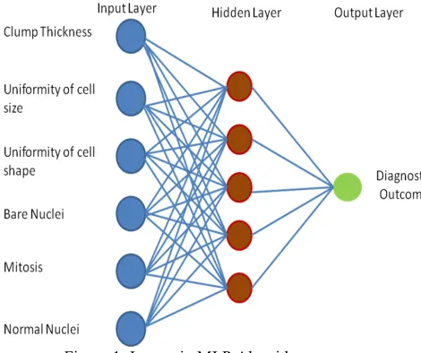
[image:2.612.326.561.210.407.2]The Multilayer perceptron calculation is a feed forward artificial neural network otherwise called the MLP algorithm. The MLP calculation can have numerous neurons in a single layer and right now can have different layers which perform calculation which thus brings about the model having a superior exactness. This calculation utilizes actuation works so as to make non-linear results. MLP comprises of an input layer, hidden layers, and an output layer. The figure beneath shows a framework of the different layers in a MLP computation.
Figure 1: Layers in MLP Algorithm
In Multilayer Perceptron Algorithm, each neuron has a bias which consists of a weight value. The value of bias in most cases will be 1.0. Every neuron in MLP will also have a weight. The values of weight will often range from 0 to 0.3. Larger weight values can increase the complexity of the model. The six input features (Thickness of the clump, cell size uniformity, cell shape uniformity, bare nuclei, Mitosis and normal nuclei) shown in figure 1 are the attributes of the dataset used for our model. The values for each of these features ranged from 1 to 10 which is shown in the table beneath.
TABLE 1: RANGE OF VALUES FOR EACH INPUT FEATURE
Features Range
Thickness of Clump 1 to 10
Cell Size Uniformity 1 to 10
Cell Shape Uniformity 1 to 10
Bare Nuclei 1 to 10
Mitosis 1 to 10
[image:2.612.319.549.575.707.2]2nd International Conference on
During the procedure, the individual estimations are sent to the first layer. This information is additionally increased with its individual weight which is determined as for the examination of its significance with different sources of input and afterward it spreads forward through the system to the neuron of the second layer which is a hidden layer. This neuron at that point utilizes an actuation capacity to process the yield. equation(1) shows this.
Output=f(x1*w1+x2*x2… … xn*wn) (1)
Here X is the input, W is the weight and f is the activation function and n speaks about the complete number of input attributes
Hyperbolic tangent function or sigmoid function can be used as activation function represented by f. MLP uses a backpropagation method for training.
B. Backpropogation Technique
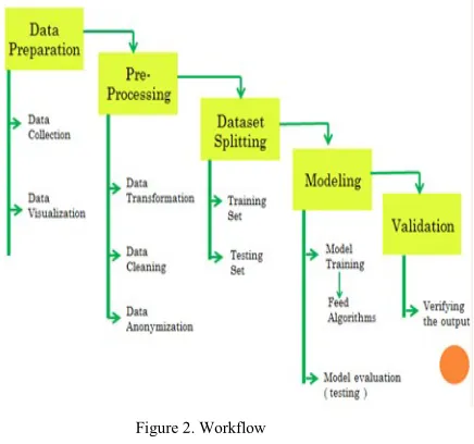
MLP calculation prepares the data set utilizing the backpropagation method. The output got after the calculation is contrasted with the output that we have in the data set. On the off chance that there is an error, the output esteem is spread in reverse through the neural system and the loads are balanced likewise. The procedure by which the loads get refreshed by considering the mistake is called online learning. When the loads are refreshed, the new indicative output esteems are determined dependent on these new loads. This procedure proceeds until the output is in greatest nearness with the normal output in the managed data set. The first phase towards developing our model is data preparation. Data preparation involves collecting breast cancer data set from hospitals or internet. The data from different datasets can also be combined in order to have a larger dataset, as larger datasets lead to more accurate results. The next step in data preparation phase is data visualization. This step involves visualizing the data in the form of correlation graph, scatter plot graph and histograms. This helps to have a better idea about the dataset.
The second phase in the methodology is data pre processing. This phase includes three steps. The first step is data transformation which includes scaling of data to a particular range, so that the model can predict the result easily. The next step in data preprocessing is data cleaning. Data cleaning involves removing unwanted data for the dataset. Unwanted data refers to data that is not required to compute the result that we require. The next step is data anonymization. This involves removing the personal details of the patient from the dataset. This involves removing ID number or name if there are any.
The third stage is dataset parting. Dataset parting includes parting the dataset into training set and testing
set. Since bigger extent of information should be prepared, 80% of information is taken for training and the staying 20% of the information is taken for testing. Preparing bigger extent of information can prompt better exactness of results.
The fourth phase is modeling. Modelling involves training the model with the help of an efficient algorithm. The algorithm we use in our model is Multilayer Perceptron Algorithm. This algorithm works on the basis of multiple hidden layers and in turn a better accuracy result can be expected. The next step in this phase is evaluation the model which can also be called as model testing. 20% of the data allotted for testing is used here. Once the testing is done, the percentage of accuracy shown by the model can be obtained.
[image:3.612.337.555.418.622.2]The fifth and final phase is the validation phase. K fold cross validation is the technique used for validation. This technique involves splitting the dataset into k groups. Suppose if k is taken as 10, then the dataset is split into 10 groups. One group will be taken for training and the remaining groups will be taken for testing and the accuracy score is evaluated. The same process is repeated taking next group for testing and the remaining for training. This process is repeated until all k groups are taken for testing. Once the cross validation is done, the model predicts if the patient has Benign tumour (non cancerous) or Malignant tumor (Cancerous). Figure 2 summarizes the entire workflow of the project.
IV PERFORMANCE FACTORS
One of the most significant and basic factor that decides the presentation of an ML model is testing. For this, we have to think about a confusion matrix. In view of the quantities got from the confusion matrix, the exactness, accuracy, review and f1score are determined.
C. Confusion matrix
Confusion matrix gives the true positive, true negative, false positive and false negative values. Here true positive and true negative shows the correct predictions made by the model and false positive and false negative shows the wrong predictions made by the model.
Table 2: Confusion Matrix
Malignant
Tumor Diagnosis Benign Diagnosis Tumor
Malignant
Tumor True Positive True Negative
Benign Tumor False Positive False Negative
D. Accuracy
Accuracy is calculated by taking the ratio of the sum of TP and TN and the value of total predictions and multiply this ratio by 100
E. Precision
Precision of malignant tumour is predicted by taking the ratio of true positive and sum of true positive and false negative. Precision of benign tumor can be calculated by taking the ratio of true negative and sum of true negative and false negative.
F. Recall
Recall of malignant tumor is calculated by taking the ratio of true positive and the sum of true positive and false positive. Recall of benign tumor is calculated by taking the ratio of true negative and sum of true negative and false positive.
G. F1 Score
The F1 score is calculated by considering the recall and precision values
V EXPERIMENTAL RESULTS AND DISCUSSION
The dataset that is utilized to prepare and test our ML model has a sum of 683 records. We split the dataset into two sections where one piece of the information is utilized for training and the other, for testing. 80% of the information is utilized for training, which brings about utilizing 546 records from the aggregate of 683 records for training the model and we utilize 20% of the information for testing which brings about thinking
about the left out 137 records for testing the presentation of the model.
We have tried the exhibition of our model utilizing five significant algorithms , for example, Gaussian Naïve Bayes, Random Forest, K Nearest Neighbor, Support vector machine (SVM) and Multilayer Perceptron (MLP) Algorithm. From the 137 records utilized for testing, the forecasts made by every one of these algorithms in given beneath:
Gaussian naïve Bayes algorithm could predict 76
malignant cases and 55 benign cases rightly and among the remaining 8 records in the testing data, 3 malignant cases were predicted as benign and 5 benign cases were diagnosed as malignant and hence the model gave an accuracy of 95.62%.
Random Forest algorithm could predict 78
malignant cases and 51 benign cases rightly and among the remaining 8 records in the testing data, 1 malignant case was predicted as benign and 7 benign cases were diagnosed as malignant and hence the model gave an accuracy of 94.16%.
K Nearest Neighbour algorithm could predict 78
malignant cases and 53 benign cases rightly and among the remaining 6 records in the testing data, 1 malignant case was predicted as benign and 5 benign cases were diagnosed as malignant and hence the model gave an accuracy of 95.6%.
Support Vector Machine (SVM) algorithm could
predict 77 malignant cases and 55 benign cases rightly and among the remaining 5 records in the testing data, 2 malignant cases was predicted as benign and 3 benign cases were diagnosed as malignant and hence the model gave an accuracy of
96.35%.
Multilayer Perceptron (MLP) algorithm could
predict 78 malignant cases and 55 benign cases rightly and among the remaining 5 records in the testing data, 2 malignant cases was predicted as benign and 3 benign cases were diagnosed as malignant and hence the model gave an accuracy of
97.08%.
2nd International Conference on TABLE 3 : PERFORMANCE OF EACH ALGORITHM WITH RESPECT TO
THE DATASET USED
Considering the accuracy of MLP algorithm a UI has been developed where the user can enter the values of the attributes which inturn displays a pop up box specifying the kind of tumor predicted by the modal.
VI CONCLUSION
As we realize that in the current framework, the PCA calculation is utilized with Classification calculations like Naïve Bayes, Random Forest, K-Nearest neighbor and Support Vector Machine and found that the precision is 95% for small dataset, yet doesn't give an equivalent/decent exactness for bigger datasets.
In this way by presenting neural network and ideas of deep learning, that is, by proposing a framework which utilizes Multilayer Perceptron algorithm we can discover whether the breast cancer tumor is malignant or benign precisely in any event, even for bigger dataset with 97% exactness.
REFERENCE
[1] Rafaqat Alam Khan, Teseer Suleman, Muhammad SajibdFarooq, Muhammad Hassan Rafiq and Muhammad Arslan Tariq.”Data Mining Algorithms for Classification of Diagnosic Cancer Using Genetic Optimization Algorithms”, 2017, Vol 17 No.12, December 2017
[2] Bharat, N. Pooja and R. A. Reddy, "Using Machine Learning algorithms for breast cancer risk prediction and diagnosis," 2018 3rd International Conference on Circuits, Control, Communication and Computing (I4C), Bangalore, India, 2018 [3] Python Machine Learning done by Sebastin Rashka and Vahid
Mirjalili
[4] "Breast Cancer Prediction via Machine Learning," 2019 3rd International Conference on Trends in Electronics and Informatics (ICOEI), by M. S. Yarabarla, L. K. Ravi and A. Sivasangari, Tirunelveli, India, 2019
[5] “Compartive Study of Machine Learning Algorithms for Breast Cancer Detection and Diagonsis”by Dana Bazazeh and Raed Shubair.,2016.978-1-15090-5306-3/ 2016.
[6] "Breast Cancer Detection Using Extreme Learning Machine Based on Feature Fusion With CNN Deep Features,"by Z. Wang et al., in IEEE Access, vol. 7, pp. 105146-105158, 2019
[7] "A Review of Breast Cancer Detection in Medical Images," by Y. Lu, J. Li, Y. Su and A. Liu 2018 IEEE Visual Communications and Image Processing (VCIP), Taichung, Taiwan, 2018
[8] "Breast Cancer Prediction via Machine Learning," by M. S. Yarabarla, L. K. Ravi and A. Sivasangari, 2019 3rd International Conference on Trends in Electronics and Informatics (ICOEI), Tirunelveli, India, 2019
[9] "A method for classifying medical images using transfer learning: A pilot study on histopathology of breast cancer," by J. Chang, J. Yu, T. Han, H. Chang and E. Park, 2017 IEEE 19th International Conference on e-Health Networking, Applications and Services (Healthcom), Dalian, 2017
[10] "Combining Deep Learning with Traditional Features for Classification and Segmentation of Pathological Images of Breast Cancer," by S. He et al., 2018 11th International Symposium on Computational Intelligence and Design (ISCID), Hangzhou, China, 2018
[11] "A Comparative Study of Breast Cancer Diagnosis Using Supervised Machine Learning Techniques," by M. Gupta and B. Gupta, 2018 Second International Conference on Computing Methodologies and Communication (ICCMC), Erode, 2018 12] "Automated Diagnosis of Breast Cancer Using Wavelet Based
Entropy Features," by K. R. and N. K., 2018 Second International Conference on Electronics, Communication and Aerospace Technology (ICECA), Coimbatore, 2018
[13] S. Lee, M. Amgad, M. Masoud, R. Subramanian, D. Gutman and L. Cooper, "An Ensemble-based Active Learning for Breast Cancer Classification," 2019 IEEE International Conference on Bioinformatics and Biomedicine (BIBM), San Diego, CA, USA, 2019
[14] N. Khuriwal and N. Mishra, "Breast Cancer Diagnosis Using Deep Learning Algorithm," 2018 International Conference on Advances in Computing, Communication Control and Networking (ICACCCN), Greater Noida (UP), India, 2018 [15] E. Halim, P. P. Halim and M. Hebrard, "Artificial Intelligent
Models for Breast Cancer Early Detection," 2018 International Conference on Information Management and Technology (ICIMTech), Jakarta, 2018
[16] N. Darapureddy, N. Karatapu and T. K. Battula, "Implementation of optimization algorithms on Wisconsin Breast cancer dataset using deep neural network," 2019 4th International Conference on Recent Trends on Electronics, Information, Communication & Technology (RTEICT), Bangalore, India, 2019
[17] L. Liu, "Research on Logistic Regression Algorithm of Breast Cancer Diagnose Data by Machine Learning," 2018 International Conference on Robots & Intelligent System (ICRIS), Changsha, 2018
[18] Y. Khourdifi and M. Bahaj, "Applying Best Machine Learning Algorithms for Breast Cancer Prediction and Classification," 2018 International Conference on Electronics, Control, Optimization and Computer Science (ICECOCS), Kenitra, 2018 [19] A. Osareh and B. Shadgar, "Machine learning techniques to
diagnose breast cancer," 2010 5th International Symposium on Health Informatics and Bioinformatics, Antalya, 2010 [20] L. Hussain, W. Aziz, S. Saeed, S. Rathore and M. Rafique,