ABSTRACT
DALEY, CAITLIN MARIE. Application of Data Mining Tools for Exploring Data: Yarn Quality Case Study. (Under the direction of Dr. Timothy Clapp and Dr. Jeff Joines).
Businesses are constantly striving for a competitive edge in the economy, and data-driven decision making is crucial to achieve this goal. Four data mining tools, principal component analysis, cluster analysis,
recursive partitioning, and discriminant analysis, were used to explore the major factors that contribute to ends
down in a rotor spinning manufacturing process. Principal component analysis was used to explore the research question about whether the large number of cotton properties used to classify cotton could be reduced to a significant few. Cluster analysis was used to gain insight about whether there were groups of gins, counties, or
classing offices that produced better raw material than others and led to less ends down. The important research question of what raw material properties were affecting ends down was explored with both recursive
partitioning and discriminant analysis. Additional research investigated the effect of cotton variety and
atmospheric conditions on spinning productivity. Each of the four data mining tools used was informative and offered a different perspective to the overall research question. Several significant factors emerged including humidity, temperature, %DP 555, and uniformity in addition to micronaire and the color properties (+b and Rd).
With these results the researcher developed an improvement plan for better control and increased spinning productivity in future operations. A designed experiment is necessary to thoroughly investigate the impact of
Application of Data Mining Tools for Exploring Data: Yarn Quality Case Study
by
Caitlin Marie Daley
A thesis submitted to the Graduate Faculty of North Carolina State University
in partial fulfillment of the requirements for the Degree of
Master of Science
Textile Engineering
Raleigh, North Carolina 2008
APPROVED BY:
_______________________________ ______________________________
Dr. Timothy Clapp Dr. Jeff Joines
Committee Chair Committee Co-Chair
ii BIOGRAPHY
Caitlin Daley started attending North Carolina State University in the fall of 2003. She completed a
Bachelor of Science in Textile Engineering with a Minor in Spanish in 2007. She continued her education in the fall of 2007 by pursuing a Master’s of Textile Engineering with a Minor in Statistics. Her background includes project work and training in Six Sigma, Design for Six Sigma, Lean methodology, errorproofing, new
product development, statistics, and various software packages. Her research interests include analytic and
iii
ACKNOWLEDGEMENTS
I would like to thank Dr. Clapp, Dr. Joines, and Dr. Thompson for their guidance and help throughout
iv
TABLE OF CONTENTS
List of Tables ... vii
List of Figures ... viii
1.0 Introduction ... 1
2.0 Literature Review & Background of Data Mining Tools ... 1
2.0.1 Introduction to Data Mining ... 1
2.0.2 Overview of Data Mining Tools ... 2
2.1 Principal Component Analysis ... 3
2.2 Cluster Analysis ... 6
2.3 Recursive Partitioning ... 10
2.4 Discriminant Analysis ... 12
2.5 Evaluation of Data Mining Tools ... 14
3.0 Yarn Quality Case Study Problem Definition ... 16
3.1 Definition of Case Study and Research Questions ... 16
3.2 Textile Yarn Spinning Background ... 17
3.3 Textile Spinning Research ... 18
3.4 Data Structure ... 20
3.4.1 Data Variable Definitions ... 21
3.4.2 Dataset Estimates ... 23
3.4.3 Cotton Variety Data ... 24
3.4.4 Temperature and Humidity Data ... 26
3.5 Data Preparation ... 26
3.6 Verification of Assumptions for Data Mining Tools ... 28
4.0 Results ... 31
4.1 Principal Component Analysis ... 31
v
4.3 Recursive Partitioning ... 44
4.4 Discriminant Analysis ... 52
4.5 Further Research ... 57
4.5.1 Cotton Variety ... 57
4.5.2 Temperature and Humidity ... 60
5.0 Case Study Discussion of Results ... 63
6.0 Recommendations and Future Work ... 67
7.0 Conclusion and Key Learnings ... 68
REFERENCES ... 70
APPENDICES ... 74
Appendix A: Nickerson-Hunter Cotton Colorimeter Diagram for Upland Cotton ... 75
Appendix B: Relationship of Trash Area to Classer’s Leaf Grade ... 76
Appendix C: HVAC Data Definitions ... 77
Appendix D: SAS Code ... 78
Appendix E: Multivariate Plots of Cotton Properties by Crop Year from SAS MULTINORM Macro ... 80
Appendix F: Univariate Skewness and Kurtosis Values by Crop Year for Eight Cotton Classification Properties .... 83
Appendix G: How-To Guide for PCA, Cluster Analysis, Recursive Partitioning, and Discriminant Analysis Data Mining Tools in JMP® Software ... 84
1. PCA ... 84
2. Cluster Analysis ... 90
3. Recursive Partitioning ... 95
4. Discriminant Analysis ... 101
Appendix H: PCA Results from AFIS Card Sliver Data ... 105
Appendix I: PCA Results from Final Yarn Testing Data ... 106
Appendix J: Hierarchical Cluster Dendrogram Results by Gin ... 107
vi
vii LIST OF TABLES
Table 2.1 Overview of Four Data Mining Tools ... 3
Table 3.1 Summary of Variable Definitions ... 22
Table 3.2 “Bad” Ends Down Quartiles by Crop Year ... 24
Table 3.3 Mardia’s Multivariate Kurtosis Values by Crop Year from CALIS Procedure ... 30
Table 4.1 Principal Component Membership of Cotton Classification Variables ... 34
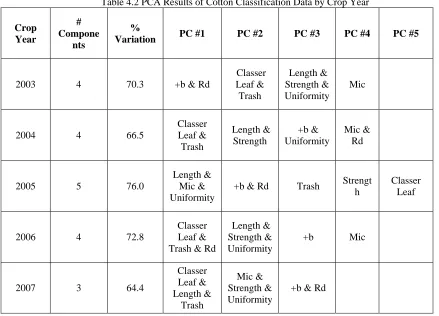
Table 4.2 PCA Results of Cotton Classification Data by Crop Year ... 35
Table 4.3 Cluster Results by County_State with Mean Values of Variables ... 39
Table 4.4 Variable Definitions and Improvement Goal ... 44
Table 4.5 Recursive Partitioning Results by Crop Year with Categorical Response for 20 Splits ... 49
Table 4.6 Recursive Partitioning Results by Crop Year with Continuous Response for 20 Splits ... 50
Table 4.7 Pairwise Correlation Results for the Number of Ends Down with the Independent Factors ... 50
Table 4.8 Confusion Matrix... 53
Table 4.9 Comparison of Stepwise Quadratic Discriminant Analysis Results by Crop Year for Two Sets of Predictor Variables ... 55
Table 4.10 Comparison of JMP® and SAS® Quadratic Discriminant Analysis Misclassification Rates with Cotton Properties and Spinning Temperature and Humidity Predictor Variables ... 56
viii LIST OF FIGURES
Figure 3.1 Yarn Spinning Process ... 18
Figure 3.2 Structure of Datasets Related to Yarn Spinning Process ... 21
Figure 3.3 Average %DP555 by Crop Year ... 25
Figure 3.4 Ends Down Average by Crop Year ... 27
Figure 3.5 Multivariate Quantile-Quantile Plot for 2003 Crop Year Data ... 29
Figure 4.1 Rotated Factor Pattern of Cotton Classification Variables ... 32
Figure 4.2 Eigenvalue Results and Scree Plot for AFIS Card Sliver Data ... 33
Figure 4.3 Scree Plot of Final Yarn Testing Data ... 34
Figure 4.4 ANOVA Results of Trash Area by Gin Cluster ... 37
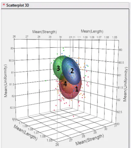
Figure 4.5 3D Scatterplot of Strength, Length, and Uniformity by Gin Clusters ... 38
Figure 4.6 Hierarchical Cluster Dendrogram and Scree Plot by State ... 40
Figure 4.7 Ends Down Average by State for 2003-2007 ... 41
Figure 4.8 K-Means Results for Four Clusters ... 42
Figure 4.9 Parallel Coordinate Plot of K-Means Clustering Results ... 43
Figure 4.10 Recursive Partitioning Output of Variable Splits ... 45
Figure 4.11 ROC Curve of Recursive Partitioning Results by Laydown ... 46
Figure 4.12 Lift Curve of Recursive Partitioning Results by Laydown ... 47
Figure 4.13 Column Contributions of Input Factors ... 52
Figure 4.14 ROC Curve ... 54
Figure 4.15 Pairwise Correlations of % DP 555 and Cotton Inc. Variables ... 57
Figure 4.16 Pareto Plot of Transformed Estimates of Ends Down Regression Model ... 59
Figure 4.17 Prediction Profiler of Input Variables’ Settings to Achieve Lowest Ends Down ... 59
Figure 4.18 Residuals Plot ... 60
1
1.0 Introduction
In today’s modern world, advances in technology have led to enormous computing and data storage
capabilities. A data management system within a company stores large amounts of data with multiple input and response variables. In fact, in 2003 WalMart recorded 20 million transactions per day into a 10-terabyte database (Shmueli, Patel, & Bruce, 2007). The analyst is faced with huge challenges in dissecting large
amounts of data and forming valuable and significant conclusions that may lead to a business advantage. Data
mining is defined as the process of selecting, exploring, and modeling large amounts of data to discover models and patterns (Giudici, 2003). More concisely, data mining is the process of extracting large amounts of information from large datasets.
Considerable amounts of data are available in all industries, and there is a huge need for tools and analysis techniques that quickly get the information in the hands of the practitioner. These tools should be
straightforward enough that all workers from the manufacturing floor up to executive leaders can implement
them and understand the results. Four data mining tools will be described including principal component analysis, cluster analysis, recursive partitioning, and discriminant analysis. A yarn quality case study will then be presented with actual data and results from using the four tools. The tool methodology and case study serve
as an example for the use of these data mining tools in the textile industry, but the tools can be applied to any data-rich problem in any industry.
2.0 Literature Review & Background of Data Mining Tools
2.0.1 Introduction to Data Mining
The recent surge in data mining research and literature highlights the importance and interest related to
this subject in today’s business world. Businesses are constantly striving for a competitive edge in the economy, and data-driven decision making is crucial to achieve this goal. Both multivariate statistics and
2
relationships among many dependent and independent variables. This type of analysis includes statistical methods that aid in data mining and simplification of large amounts of information. In relation to statistics, data
mining has been described as “statistics at scale and speed” (Shmueli et al., 2007). Knowledge discovery in databases (KDD) is another term for data mining, and it was derived from artificial intelligence research (Hand, Mannila, & Smyth, 2001). It encompasses methods to discover models and useful information in the data.
Using the four data mining tools, principal component analysis, cluster analysis, recursive partitioning,
and discriminant analysis, conclusions can be formed from a data-rich problem in any industry. Principal component analysis is used in the beginning data preparation stage to reduce the number of predictor variables to a smaller set of uncorrelated variables. Cluster analysis is used to form groups of similar observations based
on several variables to gain insight from large amounts of data. Recursive partitioning is an exploratory and interactive tool that determines optimal splits among input variables to best predict the response. Finally,
discriminant analysis is a classification and profiling tool used on continuous variables. Each of these tools is
informative and offers a different perspective to the research question of interest. A detailed review of the literature and case study examples was conducted for each of the data mining tools.
2.0.2 Overview of Data Mining Tools
The following table summarizes the four tools to be discussed in regards to the input data required, the
3
Table 2.1 Overview of Four Data Mining Tools
Tool Input Data Analysis Output Assumptions Applications
Principal Component Analysis (PCA) Highly-dimensional continuous data, multicollinear Principal components No distribution assumptions Variable reduction (data prep), exploratory Cluster Analysis Predictor and response variables (continuous/categ orical) Clusters of similar observations No distribution
assumptions Exploratory
Recursive Partitioning Predictor and response variables (continuous/categ orical) Decision tree with groupings of predictor variables that best predict response No distribution assumptions Exploratory, Classification & Regression Trees Discriminant Analysis Multiple independent continuous variables, single classification variable Linear combination of covariates that best predict group membership Predictors -multivariate normal distribution, groups - common variance-covariance matrix Classification
2.1 Principal Component Analysis
Principal component analysis (PCA) is a dimension reduction process where a large number of continuous variables are reduced and transformed to a smaller set of variables that account for most of the
variance in the original variables. A principal component is a linear combination of the optimally weighted observed variables (Lehman, O’Rourke, Hatcher, & Stephans, 2005) . By reducing the dimensionality (the
number of input variables in the model) of the dataset in the data preparation step, highly correlated variables can be represented by a single variable and the overall accuracy of the fitted model improves. The resulting
principal components are uncorrelated which is advantageous when forming a regression model because problems with multicollinear data will be avoided and the effects of individual variables can be separated
4
freedom than if all the original variables were used leading to better fitted estimates. Principal component analysis can also be used for visualization of many variables in a lower dimension to obtain more information
about a large dataset (Giudici, 2003).
The number of principal components that are extracted from the data will equal the number of original variables, but the goal is to find the few variables that explain the same information as the original, larger set of
variables. The first principal component is the linear combination of the standardized variables that lies along
the direction of maximum variance of the observations, and the second component is in the direction of the next highest variance and orthogonal or uncorrelated to the first component (Esbensen, Schoenkopf, & Midtgaard, 1994). In technical terms, the first principal component is the linear combination of the eigenvector that is
related to the largest eigenvalue of the covariance matrix and the original variable (Hand et al., 2001). The eigenvector gives the optimal weights or loadings, and the eigenvalue is the amount of variance described by a
given component for each variable (Sall, Creighton, & Lehman, 2005). The resulting principal components are
orthogonal to and independent of other predictors (Truxillo, 2005). If the measurement scales of the variables are different, standardization of the data must be done before using the covariance matrix to perform PCA so that the variability among the different measurement units of the variables does not affect the calculation of the
principal component weights. Another option to obtain standardized variables when carrying out principal component analysis is to use the scaled correlation matrix (Yang & Trewn, 2004). Sample size must also be
considered when performing PCA because it must be relatively large or at least five times the number of variables being analyzed (Lehman et al., 2005).
There are several methods of identifying the most significant components that include looking at the magnitude of the eigenvalues, using the scree plot, or comparing the percentage of variance represented by each
component. Researchers often retain components with eigenvalues greater than one, which is known as the Kaiser criterion (Lehman et al., 2005). This means that that component explains more variance than any single
5
component on the x axis in decreasing order. This plot is used to identify the “elbow” in the graph, and the number of components above this break is kept in the analysis as they are the most important. Finally,
researchers often determine prior to the analysis that a subset of components will be kept if their cumulative eigenvalue variance is at least 80% for example (Truxillo, 2005).
Once the components that account for the majority of the variability are identified using one of these
three methods, the results must be interpreted by looking at the related weight or loading coefficient between
the variables and the principal components. Loadings are a measure of the correlation between the original variable and the component and are used to compute the principal component scores (Hardle & Simar, 2003). Variables are said to load on specific components if their weight coefficients are greater than the absolute value
of .40 (Lehman et al., 2005). The principal components can also be rotated to better interpret the solution (JMP User's Guide, 2007) . It is useful to the plot the principal components against the loading of each variable to
assess the qualitative characteristics of each group (Hardle & Simar, 2003).
After the variables have been classified into common groups based on the patterns of their loadings, the components can be identified and named with the aid of a subject matter expert. For example, a six question survey to assess the volunteer attitudes of people was analyzed with principal component analysis and two
components were identified that accounted for about 70% of the total variance. The loadings were interpreted and three variables loaded on the first principal component later labeled “financial giving,” and three variables
loaded on the second component labeled “helping others” (Lehman et al., 2005). These findings enabled researchers to focus their survey efforts on these two categories.
The outcome of this analysis is a reduced set of variables that are easier to interpret and can be used for subsequent analyses. In addition, principal component analysis can be used to detect outliers in large datasets.
With the majority of the variance condensed into a few variables, a visual inspection of a histogram of the principal component scores aids in the identification of multivariate outliers that cannot be detected in 3-D
6
Principal component analysis has been used in the development of surveys or questionnaires to decrease the number of questions to a smaller set that still accounts for the same content and variability. The
response rate and efficiency of the survey will increase with a smaller number of questions that still effectively addresses the aims of the researcher’s study. For example a survey was developed to assess health care
providers’ thoughts about domestic violence in order to improve treatment methods. By using PCA the original
survey of 104 items was reduced to six principal components or content domains made up of 39 total items
(Maiuro, 2000). This new survey more accurately and efficiently assessed health care providers’ opinions. It extracted the same information that the original 104 item survey did, and the results led to a better treatment plan for victims of domestic violence.
Another application of principal component analysis is as a preparatory step for regression analysis. Collinearity among input variables leads to unstable models, so principal component analysis is a method to
obtain independent variables to use in the analysis. An international math study was completed to investigate
skills, perceptions, and behaviors of middle and high school age students. Data was collected on many variables with the goal of predicting the students’ math test scores. Twelve variables were analyzed and found to be highly correlated, so principal component analysis was conducted to obtain a set of independent, surrogate
predictors to use in the regression analysis. Two principal components were identified and input into the regression analysis to more accurately predict math test scores (Truxillo, 2005).
2.2 Cluster Analysis
Cluster analysis is the process of identifying unknown groups in observations by minimizing the
within-cluster variation and maximizing the between-cluster variation. It is an exploratory method to identify similar objects in large datasets, and the number and names of the groups are not known beforehand (Sall et al.,
2005). It is an unsupervised learning method to determine the natural groupings in the data as there are no reference variables with known levels or classifications. On the other hand, discriminant analysis discussed
7
Truxillo, 2005). Cluster analysis is often used in market based research for customer segmentation and
structure analysis and is a very common descriptive data mining method (Shmueli et al., 2007 ; Giudici, 2003).
To complete cluster analysis the distance between observations and between clusters needs to be determined. Several measures exist to calculate the distance between observations including the Euclidean distance, standardized Euclidean distance (Pearson method), correlation-based similarity, Mahalanobis distance,
Manhattan distance, and maximum coordinate distance. The standardized Euclidean distance is most
commonly used although it doesn’t account for correlation between variables and is very sensitive to outlying values (Shmueli et al., 2007). Linkage methods are used to calculate the distance between clusters and include minimum distance (single), maximum distance (complete), average distance, centroid distance, and Ward’s
methods (Yang & Trewn, 2004 ; Shmueli et al., 2007). Minimum distance (single), maximum distance (complete), and average distance calculate the distances between each observation of the two groups being
compared. The centroid method calculates the centroid of each group for comparison, and Ward’s method
analyzes variance within and between the clusters rather than using a distance measure (Giudici, 2003). Using these techniques to calculate the between observation and between cluster distances, there are
then several methods to perform the actual cluster analysis that include normal mixtures, self-organizing maps,
hierarchical cluster, and k-means (Sall et al., 2005). The objective of these methods is to get internal cohesion and external separation among the groups (Giudici, 2003). The two general types of clustering algorithms are
hierarchical and nonhierarchical (k-means) methods that are discussed in detail below. Once the cluster analysis has been completed, the results are then interpreted to determine the names and characteristics of the
clusters (Yang & Trewn, 2004). The researcher must work closely with an expert in the discipline when classifying and labeling the clusters.
The hierarchical method is commonly used and easier to implement with smaller datasets. In this method the number of clusters obtained may range from one to the number of observations present where each
8
combining observations with the closest distance until all observations are combined into one large cluster at the end. The divisive hierarchical method is the opposite and begins with one large cluster of all the observations.
The large cluster is divided into smaller clusters at each step until each observation is in a cluster by itself (Shmueli et al., 2007). An output of hierarchical cluster analysis, either agglomerative or divisive, is a dendrogram which is a tree-like depiction of each observation, its clustering sequence, and the distances
between clusters. Using a similarity measure or cutoff line on the chart, the number of clusters can be identified
(Sall et al., 2005). The researcher must be cautious when blindly using a cutoff line or “tree cut” on the dendrogram because it may not accurately depict the number of clusters (Kettenring, 2006). A scree plot is also used to show the distances between clusters and a natural break in the curve is an estimate for the number of
clusters that represent the data. Subject matter experts should review the cluster results for understanding and
interpretation.
The nonhierarchical or k-means method is used for large data sets and starts with the identification of
the number of clusters (k). Nonhierarchical methods are quicker than the hierarchical methods because a distance matrix does not have to be calculated for each partition (Giudici, 2003). The computer software calculates the k cluster centroids or seeds at random points in the dataset. Each observation is assigned to the
closest cluster, the k centroids are recalculated based upon the new assignment, and the process repeats until no observations are reassigned. Because of the challenge of predicting the number of clusters beforehand in this
method, the number of data clusters found in the hierarchical method could be used and input into the k-mean method for further analysis (Yang & Trewn, 2004). Different values of k can be iteratively analyzed to
determine the best clustering results. Problems can occur with outliers because the k-means analysis may lead to small clusters of these extreme values with large clusters containing the majority of the observations
(Giudici, 2003).
Both clustering methods were used to look at risk and protective factors among middle school students
9
were carefully considered and selected on criteria important to the aims of the study. The data was standardized and hierarchical analysis was first performed. The results from the dendrogram were used to further analyze
three, four, and five clusters in the subsequent k-means analysis. Four clusters were found to best describe the differences in the data among the students and were broadly labeled as protected, high-risk, coping, and disconnected. The researchers than validated the differences between these clusters through chi-squared and
analysis of variance methods (Anthony, 2008). This application highlights the complementary nature of these
two clustering algorithms, the hierarchical and k-means methods.
Applications of cluster analysis exist in many industries such as marketing to describe different customer segments, in psychology to discover personality types based on surveys, in psychiatry to create
categorizations of mental illnesses, in meteorology to identify spatial pressure patterns for climate studies of the atmosphere, and many other examples given below (Hardle & Simar, 2003 ; Hand et al., 2001). Market and
political forecasters commonly use zip codes to group neighborhoods by their preferences (Shmueli et al.,
2007). Cluster analysis could be employed in the new product development process. Different brands and products on the market could be classified to identify the competitive and successful clusters of products. The business can then assess the impact of its new product on this market cluster structure and its potential success.
Otherwise, the business can begin the design process anew for the development of a unique and innovative product that fills a niche in the cluster structure (Punj, 1983).
Cluster analysis has also been used in healthcare. Several years ago clustering analyses were done with nursing survey data to discover more information about stress and burnout. The researchers found that
stress is more related to the work environment and overall workload than with the degree of specialization on the clinical service unit. Also it was determined that more psychological damage results from conflict with
physicians than problems with other nurses (Hillhouse & Adler, 1997). Another study looked at chronic senility in patients to improve the medical care they were receiving. The researcher investigated patients’ revisit
10
patients with poor health so efforts were directed at more effective treatment for overall improved health and wellbeing. The second cluster of patients had a low revisit frequency, and administrators targeted their efforts
to increase these patients’ customer satisfaction and business (Cheng, 2006). In this case researchers were able to use the results from the cluster analysis to better serve their patients.
2.3 Recursive Partitioning
Recursive partitioning is a method that splits data to find groupings of input variables that best predict
the response. It is also referred to as decision trees or the CARTTM program (classification and regression trees). This method recursively fits all possible splits to find the optimum partition that maximizes the difference in the responses between the two branches. If the response is continuous, the splits are made to
maximize the difference between the means by looking at the squared errors. If the response is categorical, the estimated probability for each response level is calculated and the splits are made to maximize the
likelihood-ratio chi-square statistic (JMP User's Guide, 2007) . The tree is made up of stepwise, univariate binary
decisions that lead to simple classification rules that can be applied in practical applications (Hand et al., 2001). For instance, a set of questions to ask patients during triage can be formed from a table of symptom and disease diagnosis data. Once the data partitions have been made, the resulting “leaves” at the terminal nodes of the
decision tree label the most likely class and its associated probability (Giudici, 2003). It should be noted that association not causality can be determined from this exploratory modeling method.
In order to avoid problems with overfitting the data, different stopping criteria and pruning methods have been developed to eliminate weak and unimportant splits (Shmueli et al., 2007). The ideal decision tree
has minimal leaves to aid in interpretation of the predictive model and at the same time lots of leaves to increase the accuracy of the model. Stopping rules can include criteria about the number of leaves or the number of
steps, or the analysis may stop when the decrease in impurity or heterogeneity is too small. In a study for example, researchers defined a terminal node if the leaf had less than 25 observations or the increase in the
11
subtree that minimizes a loss function or cost-complexity measure (Giudici, 2003). The tradeoff between the misclassification error and the number of nodes in the tree is crucial in order to model the patterns but not the
noise in the data (Shmueli et al., 2007). Therefore, researchers often fit several different models on the training data and then assess their performance with the validation data by looking at the R-squared value and the lift or ROC curves (Gaudard, Ramsey, & Stephens, 2006).
Recursive partitioning is a useful tool for variable subset selection and does not require any
transformation of the variables since there are no distribution assumptions for the analysis. Outlying values may significantly alter the results, so data exploration is an important step to complete prior to the analysis (Giudici, 2003). This method requires a large dataset to form significant conclusions from a classifier, but
recent research has investigated the use of random forests to create many classification trees from a smaller dataset. These results could then be combined for an improved conclusion (Shmueli et al., 2007). In addition,
exploratory recursive partitioning can be a helpful method to determine factor levels for a subsequent designed
experiment by assessing the partition split values and probabilities (Gaudard et al., 2006).
A specific application of recursive partitioning was to look at a sample of patients that underwent treatment in a Radiation Therapy Oncology Group (RTOG) brain metastases trial. Cancer patients often
develop brain metastases and doctors struggle with selecting the patients that will benefit the most from an aggressive treatment. A sample set of 1200 patients with twenty-one variables each were analyzed using
recursive partitioning to evaluate the effectiveness of the treatment interventions. Two significantly different groups of patients were found that had survival rates of 7.1 and 2.3 months respectively. Based on the
characteristics and variable levels of these two groups obtained from the partition analysis, future clinical trials will be redesigned and doctors will target patients that have a better survival rate for aggressive treatments
(Gaspar, 1997).
Another application of recursive partitioning was in the field of meteorology. Scientists in Australia
12
minimum cost-complexity. This model was then applied in case studies throughout Australia to assess its effectiveness in different climate regions (Schnur, 1998).
Recursive partitioning was used in a manufacturing setting to investigate factors that may have contributed to banding defects in a printing process. Banding occurs when there are irregularities in the cylinder that transfers ink to the paper and therefore causing imperfections in the final product. The process
team brainstormed thirty-nine potential factors that included both nominal and continuous variables. Due to the
number of variables, their type, and the difficulty in using a specific statistical tool with several assumptions, recursive partitioning was used to explore the conditions that may lead to a printing defect (Ramsey, Stephens, & Gaudard, 2005).
2.4 Discriminant Analysis
Discriminant analysis, also known as Fisher’s rule, classifies units into predefined groups based on
similar characteristics (Giudici, 2003). The goal of this analysis is to determine which variables best predict
group membership. This analysis is often considered a multivariate generalization of logistic regression (Truxillo, 2005). A linear discriminant function is used as the prediction criteria or “cutoff” score for
classifying two groups, and Mahalanobis distance is used when categorizing multiple groups (Yang & Trewn,
2004). The discriminant function obtained is very useful to predict the classification of future observations. The major assumptions in discriminant analysis are that the predictors are from a multivariate normal
distribution, linearly related, and the categorical groups have a common variance-covariance matrix (Esbensen et al., 1994). Skewed data can considerably affect the resulting analysis so data transformations may be needed,
however the method is more robust for large sample sizes. Quadratic discriminant analysis can be used instead of linear discriminant analysis if the covariance structure is significantly different (Shmueli et al., 2007). The
quadratic discriminant analysis uses a separate estimate of covariance for each group rather than the pooled estimate that is used in the linear method (Truxillo, 2005). Research has shown that discriminant analysis is
13
The general method of discriminant analysis is to classify observations into groups that are the closest distance away. Different distance measures can be used to calculate the distance from the observation to the
mean (for a single variable class) or the centroid (vector of means for two or more variables) of the class. The Euclidean distance is commonly used although it is not a standardized distance, does not account for variance of the variables, and disregards any correlation between the variables. An alternative is to use the Mahalanobis
distance which takes into account the variability and correlations of the variables. Once the distances have been
calculated, a linear classification function with weighted discriminatory variables is found that maximizes group separation. A classification score is computed for each observation and the observation is grouped in the class for which it has the largest score, corresponding to the smallest distance from the class (Shmueli et al., 2007).
The discriminant functions are determined from the test data and should be validated with a validation sample to assess the classification error rate and the fit of the model (Truxillo, 2005). A practical consideration the
researcher should make when using discriminant analysis is the expected cost of misclassification and the
complexity related to the classification decision. Information about unequal misclassification costs can be added to the functions in order to minimize the expected misclassification costs (Shmueli et al., 2007).
Stepwise discriminant analysis can be used to find the order of the variables that best predict group
membership. Statistical criteria such as the alpha level are used to add or remove variables to the model (Truxillo, 2005). These results can be used when forming a regression model or simply to reduce the number of
variables to the few, statistically significant predictors.
An application of discriminant analysis is in categorizing current and potential credit card holders into
“good” and “bad” groups based on variables such as education level, salary, family size, and credit rating among others. By developing a discriminant function based on these variables, potential credit card holders can
be screened and classified as a “good” or “bad” customer. Businesses can adjust their marketing and recruiting plans to increase revenue for the company by targeting their efforts towards desirable customers (Yang &
14
responses from a 12-item questionnaire related to gambling. The participants were identified as one of the following types of gambler: binge, steady, or control. Two discriminant functions were identified from the
analysis that maximized the distances between the group centroids. The first discriminant function seemed to divide the binge and steady gamblers while the second function separated the control and steady gamblers (Truxillo, 2005). These resulting functions based on the twelve variables were extremely useful for researchers
in identifying people with potential gambling problems.
2.5 Evaluation of Data Mining Tools
When analyzing classification and prediction results, there are several methods to assess the performance of the tool employed. The classification or confusion matrix shows the correct and incorrect
classifications for a specific dataset by assessing the actual and predicted class of observations. The number of correct classifications is displayed on the diagonal, and the overall error and accuracy can then be calculated
from this matrix. Other common metrics calculated include sensitivity and specificity. Sensitivity is the
probability that the predictor correctly classifies an observation, and specificity is the probability that the predictor correctly rules out an observation. The Receiver Operator Characteristic (ROC) curve is often used to depict the relationship between false-positive or false alarm on the x-axis (1-specificity) and true-positive or hit
rate on the y-axis (sensitivity) rates, and the area under the curve is used to evaluate this relationship. An area of 1 corresponds to a perfectly fitting model with accurate discriminatory power while an area of .5 corresponds
to a model fitting chance alone. The ROC curve highlights the predictive accuracy of the model and is based on the confusion matrix (Giudici, 2003). Both the classification matrix and ROC curve are used to assess
discriminant analysis results, and the ROC curve is also used to find the best fitting model for recursive partitioning.
A lift chart is similar to the ROC curve and is used to look at the specificity versus the cumulative number of observations to compare the performance of the model with different portions of the population
15
show the relative improvement of the fitted model. Lift curves are commonly used to assess the many different splits and fitted models used in recursive portioning.
A consideration when selecting a model that accurately describes the data is the bias-variance trade-off. Bias is the systematic error between the expected value and true observation and is related to the model approximation. Variance is the random and data-driven component of error (Hand et al., 2001).
Cross-validation can be used to find solutions to the bias-variance dilemma through different model selection criteria.
For this method the dataset is usually divided into three parts for analysis: training, validation, and testing. The training data is used to fit the model, and the model is then selected using the validation data. The prediction error will be calculated using the test data. Another approach is the k-fold cross-validation in which k subsets
of data are formed from the dataset. The model is fit k times and one subset is excluded each time which is used to calculate the prediction error (Giudici, 2003). Cross-validation is commonly used with both recursive
partitioning and discriminant analysis to assess the fit of the training model on the validation or hold-out data,
and classification error statistics can be calculated.
In addition to these methods for assessing the results from the classification and prediction tools, some basic methods or statistics can be used to evaluate the exploratory tools. For PCA the results can be quantified
by looking at the cumulative percent variation represented by the eigenvalues. For cluster analysis, the clusters can be verified by looking at the spread of the cluster observations across several variables and an analysis of
variance conducted to see if the clusters are statistically different. An R-squared value, the proportion of variance explained by the model, is often shown for recursive partitioning, and a graph showing this value
16
3.0 Yarn Quality Case Study Problem Definition
3.1 Definition of Case Study and Research Questions
After the researcher established an understanding of the four data mining tools and how they have been
used in different applications, a case study was chosen to use these methods to solve a real problem in industry. A specific textile manufacturing plant was studied with the research aim to improve yarn productivity by
focusing on ends down in the production of cotton yarn in the open end spinning process. An ends down is defined as a yarn break in the final production process where cotton sliver is spun into cotton yarn. Ends down
lead to decreased efficiency and profit because they are an interruption in the manufacturing process that must be repaired before production can be continued. By exploring and analyzing the many different variables
concerning the raw materials and spinning processes, the researcher hoped to obtain an understanding of the major factors that contribute to ends down to develop an improvement plan for better control and productivity
in future operations.
The overall objective of the case study was to determine what factors were driving ends down by using
the four data mining tools to improve the overall efficiency in the spinning process. Specific research questions were identified that could be addressed by each of the statistical tools and result in data-driven decisions to
guide continuous improvement. Principal component analysis was used to explore the research question about whether the large number of cotton properties used to classify cotton could be reduced to a significant few.
Cluster analysis was used to gain insight about whether there were groups of gins, counties, or classing offices that produced better raw material than others. The important research question of what raw material properties
were affecting ends down was explored with both recursive partitioning and discriminant analysis. Recursive partitioning helped define a decision tree and factor levels that would lead to decreased ends down, and
discriminant analysis yielded a classification function with material properties as inputs to predict the number of ends down as the outcome. Additional research investigated the effect of cotton variety and atmospheric
17
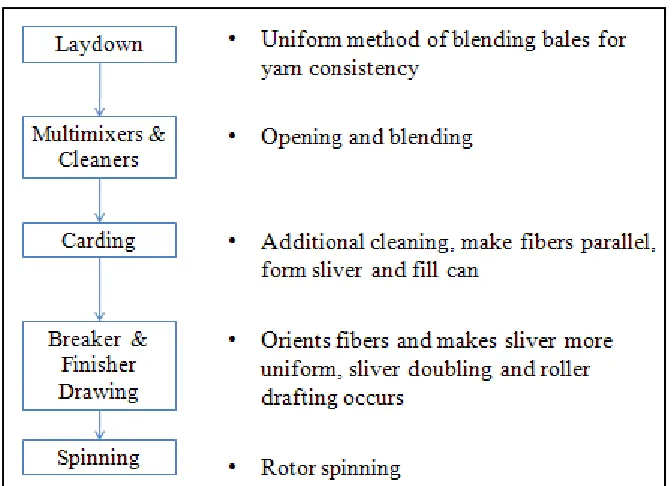
3.2 Textile Yarn Spinning Background
Open-end rotor spinning is the process from which a bale of raw cotton is blended, cleaned, processed,
and spun into yarn. The figure below depicts the yarn spinning process. First, laydown machines uniformly blend ninety bales of cotton with varying properties to achieve an “average” laydown with a wide distribution of properties. Multimixers and cleaning machines open and blend the cotton to decrease trash and any foreign
particles that may be leftover from the ginning process. The laydown is then processed in the carding machines
where the fibers are further cleaned, rid of entanglements, and made parallel into cotton sliver, a ropelike extension of the cotton fibers. The drawing machines orient and cross-blend the fibers and make the sliver more uniform through doubling. The doubling process is where six slivers are combined to decrease the
coefficient of variation of the output sliver strand; a low coefficient of variation value corresponds to a more uniform thickness profile of the sliver. Finally, the sliver is processed in the open-end rotor spinning machines
where yarn is produced and wrapped up in packages. The actual yarn formation occurs in the spinbox, and the
spinning and winding steps are combined into one step. The specific manufacturing plant in this study consumes about 90,000 bales of cotton per year and produces mainly 100% cotton with a cotton count of 18 hanks per pound (Ne=18). A hank is equivalent to 840 yards, and a larger cotton count corresponds to a finer
18
Figure 3.1 Yarn Spinning Process
3.3 Textile Spinning Research
The researcher studied the textile literature for the influence of cotton characteristics on yarn quality
and factors that may affect spinning productivity. First, the researcher focused on studies that relate cotton fiber characteristics to yarn quality. For 100% cotton yarns strength, fineness, and length are the most important
fiber properties for rotor spun yarn (Bradow, 2000). A study was done to specifically investigate the effects of fineness and strength on open-end yarn properties, and it was found that low micronaire cotton was more
important than strength to the resulting yarn strength (Simpson & Murray, 1978). For blended yarns friction is an additional important property because it aids in fiber cohesion. In regards to strength, fineness, and length
researchers have shown that fiber length is primarily a genetic trait that is directly related to yarn fineness, strength, and spinning efficiency (Bradow, 2000).
A study was completed to look at the effect seven fiber properties (micronaire, length, length uniformity, strength, greyness, yellowness, and trash grade) had on the strength of open-end rotor spun yarns.
19
yarn strength. In addition they found there is a strong positive relationship between micronaire and length uniformity, strength and length, and a strong negative relationship between micronaire and length. The
researchers highlighted the lack of significance of the effect of fiber length on yarn strength (Ethridge, Towery, & Hembree, 1982).
Next, the researcher focused on known factors that affect spinning productivity defined as the number
of ends down in the production. An experiment was conducted to investigate ends down in a ring spinning
process of cotton yarn. It was found that large amounts of short fiber content was the most significant factor affecting ends down followed by span length, micronaire variability, and the number of bales per laydown. Short fiber content was defined as the percentage of fibers shorter than 12.5 mm in length (Backe, 1986).
Another study was done to determine the effect of blend, twist factor, and fineness of cotton on spinning productivity. The largest ends down rate was seen with 100% coarse and 100% low-strength cotton at low twist
factors, and lower ends down were related with fine fiber cotton (Simpson & Murray, 1978). Micronaire is an
important factor that affects both the yarn quality and spinning productivity where fine fiber cotton leads to lower ends down. Finally, a research study was conducted to investigate the effect of feed sliver moisture content on rotor spinning performance. It was found that high moisture content in the feed sliver leads to
decreased ends down but negatively impacts yarn evenness and elongation as the number of imperfections increases (Basal & Rust, 2001).
The impact of the atmospheric conditions on spinning productivity was then researched. A study was done to examine the effects of a direct conditioning system on spinning productivity under two different
scenarios of cold/dry and warm/humid. The warm/humid conditions were found to lead to more ends down because of fluctuations in the abrasion between the fiber and metal of the open end machine. In addition, the
number of yarn imperfections and cotton stickiness increased. It was concluded that temperature and humidity have a larger effect on yarn performance than yarn quality (Artzt P., Herter T., & Preininger H., 1990). The
20
The stickiness of cotton and sugar accumulation on the machinery leads to decreased spinning productivity because the frictional forces are increased resulting in more machine wear (Hequet, 2005).
Fiber color can be traced back to how the cotton was grown and ultimately related to fiber quality and even spinning productivity. For example, white fibers with high Rd values are more mature and of higher quality than dull and yellow fibers that resulted from bad environmental conditions. The ultimate cotton fiber is
white as snow, strong as steel, as fine as silk, and as long as wool (Bradow, 2000). Factors that negatively
affect the ideal color properties include weather, insect damage, foreign matter contamination, and excessive moisture and temperature levels during storage. These damaging effects of the environment on the color of cotton later lead to decreased spinning productivity. The color properties can also affect other processes such as
dye uptake and the application of finishing treatments (The Classification of Cotton 2001) .
3.4 Data Structure
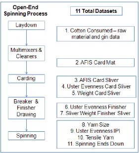
After definition of the research questions and review of the textile yarn spinning process, eleven total
datasets were obtained with around 500,000 observations and nearly one hundred different variables detailing information about the cotton classification properties, production process, and quality of the end yarn product (see Figure 3.2 below). There were approximately 350,000 cotton bales, 4300 laydowns, and 300 gins studied
in the cotton data from October 2003 to May 2008. The researcher was faced with lots of information but used data mining tools to explore the data to find patterns and useful information for quality improvement at the
21
Figure 3.2 Structure of Datasets Related to Yarn Spinning Process
3.4.1 Data Variable Definitions
The majority of the research focused on the cotton classification properties and their effect on spinning
ends down in the final process step. Before analyzing the data, an understanding of the variables and their definitions was necessary in order to comprehend the results and form meaningful conclusions. The United
States Department of Agriculture has several Classing offices throughout the US that classify the bales of cotton based on several parameters including fiber length, length uniformity, strength, micronaire, color, trash area,
and classer leaf grade. Two samples of fibers are taken from each bale for the testing which primarily occurs on the high volume precision instrument (HVI) machines, although the leaf grade is determined manually (The
22
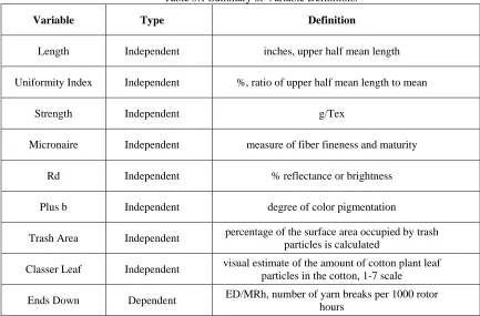
Table 3.1 Summary of Variable Definitions
Variable Type Definition
Length Independent inches, upper half mean length
Uniformity Index Independent %, ratio of upper half mean length to mean
Strength Independent g/Tex
Micronaire Independent measure of fiber fineness and maturity
Rd Independent % reflectance or brightness
Plus b Independent degree of color pigmentation
Trash Area Independent percentage of the surface area occupied by trash particles is calculated
Classer Leaf Independent visual estimate of the amount of cotton plant leaf particles in the cotton, 1-7 scale
Ends Down Dependent ED/MRh, number of yarn breaks per 1000 rotor hours
Fiber length is the upper half mean length (the average length of the longer half of fibers) and is reported in inches with a short fiber defined as less than 0.99 inch. Length uniformity or the uniformity index is the ratio of the mean length to the upper half mean length of the fibers, and 77% or less is a very low degree of
uniformity. The strength of a fiber is the amount of force in grams necessary to break one tex unit of fibers, and
a strength value less than 23 grams per tex characterizes a weak fiber. A tex is the weight in grams of 1,000 meters of fiber. Micronaire is a gauge of the fineness and maturity of the fibers with a smaller micronaire value corresponding to finer fibers. The color of fibers is measured by the degree of reflectance and yellowness.
Reflectance (Rd) is the percentage reflectance or brightness of the fibers, and the yellowness measure (+b) is the amount of color pigmentation. These two values are plotted on the Nickerson-Hunter cotton colorimeter
diagram, and the fiber sample’s three-digit color code is determined by the intersection of these two values on
23
present in the sample on a scale from one to seven with seven corresponding to higher trash content. Although the trash area and classer leaf grade are measured separately, there are observable correlations between the two
measures (see Appendix B) (The Classification of Cotton 2001) .
Short Fiber Index was an additional variable present in the material data that the USDA Classing offices do not measure. It is a function of the uniformity and length of the fiber and therefore an indirect
measurement that is highly correlated with both of these variables. Therefore, it was not considered in the
analyses because the uniformity and length variables sufficiently described the cotton material properties. Ends down in the manufacturing plant are measured as the number of yarn breaks per 1000 rotor hours, and this variable was used as the main outcome measure of the process (dependent variable). Other available
data included information from intermediate processes such as the card and drawing sliver and the physical yarn testing data.
3.4.2 Dataset Estimates
To address the main research question of the impact of raw material on spinning productivity, two datasets had to be joined, Cotton Consumed (raw material) and Spinning Ends Down. There was no common
identifier between the two datasets and only limited data available about the process flow rate; therefore, the researcher attempted to define an approximate time between laydown and spinning in order to merge the
datasets based on production time. The average production rate of the spinning plant was 855,000 pounds per week with one laydown weighing approximately 45,000 pounds, and so the weekly production was about
nineteen laydowns. A continuous spinning operation was assumed with 168 working hours per week which led to the approximation that each laydown takes about 8.8 hours from laydown to spinning.
Considering the production and efficiency rates and work in production (WIP) levels, a more detailed analysis was done that led to a calculated 8.4 production hours per laydown. From these results and due to the
fact that the data is only averaged and available daily, the researcher assumed a two day moving average estimate from the laydown to ends down. This estimate was confirmed with the project sponsor and then used
24
Due to the vague estimate that was made for the time between the raw material and ends down data and the many other potential factors that could impact the process, only speculative evidence can be determined
for the analyses and all conclusions are exploratory. In the future a designed experiment should be conducted to track a specific laydown of cotton through the spinning process to collect more reliable data. Precise labeling and tracking of the cotton material would be necessary throughout the process. This tracking requires
considerable effort due to the nature of the spinning process that involves lots of blending and different steps to
yield uniform properties.
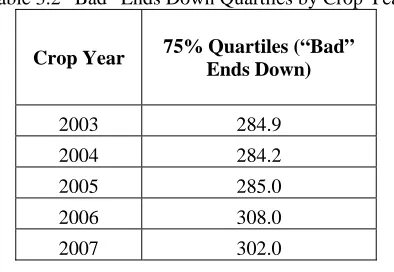
In addition to the time estimate, the researcher made an assumption about “good” and “bad” levels of ends down in order to recode the continuous values into a categorical variable. For each crop year, the number
of ends down were coded as “bad” if they were greater than the 75th percentile (see table). This classification of the spinning outcome as “good” or “bad” enabled a categorical response to be used in fitting models for
recursive partitioning and discriminant analysis.
Table 3.2 “Bad” Ends Down Quartiles by Crop Year
Crop Year 75% Quartiles (“Bad” Ends Down)
2003 284.9 2004 284.2 2005 285.0 2006 308.0 2007 302.0
3.4.3 Cotton Variety Data
At the suggestion of the project sponsor, the researcher investigated the effects of a specific cotton
variety on US cotton properties in general and then in relation to the specific case study. Based on the
sponsor’s process knowledge and industry experience, he hypothesized that increasing percentages of Deltapine
25
pest control to cotton, and RR (Roundup Ready) is the genetic engineering process to enable cotton to be safely treated with herbicides (glyphosate) that kill harmful weeds. The amount of Deltapine variety grown has
steadily increased over the past several years (see figure below). It represents a significant portion of the total US Upland cotton acreage and is the most planted cotton product (Deltapine, 2008) .
Figure 3.3 Average %DP555 by Crop Year(Agricultural Marketing Service, 2002-2007)
Six years of USDA cotton variety data by state for AL, FL, GA, LA, MS, and SC was analyzed and compared to the resulting crop quality summary data from Cotton Incorporated. The researcher was ultimately
looking for any correlations and relationships between this specific Deltapine cotton variety factor and the resulting cotton classification properties. After the collection of the USDA and Cotton Incorporated data, the
percentage of DP 555 cotton variety data by state was related to the material and spinning ends data for the specific case study. The USDA data concerning the percentage of DP 555 grown per crop year per state was
added to the cotton data based on the state where the cotton bale was ginned. The cotton variety data was added for all ten ginning states represented in the case study dataset: AL, AR, FL, GA, LA, MO, MS, NC, SC, and
2002 2003 2004 2005 2006 2007
% DP 555 0.5 26.3 43.2 48.6 54.6 64.3
0.0 10.0 20.0 30.0 40.0 50.0 60.0 70.0
%
DP
555
26
TN. The percentage of DP 555 and its effect on the cotton classification properties and the number of ends down was considered in recursive partitioning, discriminant analysis, and a separate regression analysis.
3.4.4 Temperature and Humidity Data
Temperature and humidity data later became available as part of the case study. The researcher wanted
to determine if the temperature and humidity inside and outside the manufacturing plant had any influence on
spinning productivity in terms of ends down. The data was measured every minute in the plant but it was compiled to a daily average to match with the spinning data. This environmental data was available from the cleaning, carding, drawing, and spinning zones within the plant and the researcher chose to focus on the zones
associated with the spinning production (see Appendix C). The average temperature and humidity values in spinning were calculated for these three zones. The effects due to these spinning conditions in addition to the
outside temperature and humidity variables were considered in both recursive partitioning and discriminant
analysis.
3.5 Data Preparation
After determination of the research questions, data structure, and variable definitions the researcher began preparing and exploring the data for analysis. This preliminary data preparation step is critical for any
conclusions that are ultimately made because of the well-known reality that bad data input into the analysis tools will only lead to bad results, the “garbage-in, garbage-out” phenomenon. The data should be cleaned by
identifying outliers and missing data. It is helpful to graphically explore the data via histograms, scatterplots, or other methods to observe the spread of the data and to detect any collinearity or correlation among variables.
Specific statistical assumptions may need to be checked such as multivariate normality and equality of the variance-covariance matrices. Depending on the results of the normality tests, the data may need to be
27
validation datasets, typically a 70/30 split. The models can then be tested on the validation data to avoid overfitting problems.
The researcher initially explored the distribution of the data using histograms, scatterplot matrices, and pairwise correlations between factors. As mentioned above, the Short Fiber Index variable was collinear with uniformity and length so it was not included in further analyses. By definition, variables are collinear if they
are highly correlated (Truxillo, 2005). The researcher also looked at the raw material and ends down trends
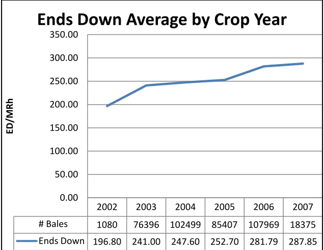
over time and noticed significant differences by crop year, the year the cotton was grown. Therefore, the five years of data was divided by crop year into manageable groups to more accurately investigate important factors (see figure below). Since there were so few observations and only four days of available data for the 2002 crop
year, it was eliminated from further crop year analyses.
Figure 3.4 Ends Down Average by Crop Year
2002 2003 2004 2005 2006 2007 # Bales 1080 76396 102499 85407 107969 18375 Ends Down 196.80 241.00 247.60 252.70 281.79 287.85
0.00 50.00 100.00 150.00 200.00 250.00 300.00 350.00
ED/MRh
28
3.6 Verification of Assumptions for Data Mining Tools
Principal component analysis, cluster analysis, and recursive partitioning do not require any specific
statistical assumptions because they are exploratory tools but significant outliers were eliminated from the data prior to use of these analyses. Discriminant analysis does require the assumptions of multivariate normality and a common variance-covariance structure. SAS® software was used to check these assumptions for each dataset
by crop year, and specifically the %MULTINORM macro to test multivariate normality, the CALIS procedure
to check the multivariate kurtosis and skewness, and the DISCRIM procedure to test the homogeneity of the covariance matrices (see Appendix D for SAS code used).
The %MULTINORM macro is a procedure to check the multivariate normality of several variables.
The assumption of multivariate normality means that the joint distribution of the variables is normal in addition to each variable being univariate normal (Truxillo, 2005). First, the univariate procedure was used to check
univariate normality by examining the quantile-quantile plots of each of the eight cotton classification variables
(mic, length, strength, +b, Rd, trash area, uniformity, classer leaf). These plots showed varying trends and distributions due to the nature of some of these variables, and univariate normality could not be assumed. However, because of the exploratory nature of this data mining analysis, the overall normality assumption was
not rejected and further checks on the multivariate distribution were completed. The %MULTINORM macro was then used to look at the multivariate normality. Output from the macro includes a multivariate
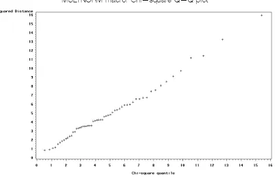
quantile-quantile plot of the squared Mahalanobis distances of the observations from the centroid against the chi-squared quantiles. The data is multivariate normal and distributed as a chi-squared distribution when these plotted
values are close to a diagonal straight line. For example the figure below for data from the 2003 crop year shows a multivariate normal distribution because the points are approximately centered on a diagonal line.
29
Figure 3.5 Multivariate Quantile-Quantile Plot for 2003 Crop Year Data
In addition to checking the univariate and multivariate quantile-quantile plots, the skewness and
kurtosis of the data were investigated. Skewness is a measure of the lack of symmetry of the data, and kurtosis is a measure of the peaked or flat nature of the data relative to the normal distribution. Kurtosis problems have
a larger impact on the multivariate normality of a dataset than skewness (Truxillo, 2005). The CALIS
(Covariance Analysis and Linear Structural equations) procedure was used in SAS® to assess these multivariate
measures. The univariate kurtosis and skewness values showed no significant nonzero values or obvious departures from normality (see Appendix F). The table below shows Mardia’s multivariate kurtosis statistics
for each crop year, and in general there were no significant nonzero values except for the outlier in 2005. A detailed analysis of this dataset was later conducted and it was found that all values for the classer leaf variable
30
multivariate normal and the exploratory data analysis could be carried out without major data transformations based on the multivariate quantile-quantile plots and the kurtosis and skewness statistics.
Table 3.3 Mardia’s Multivariate Kurtosis Values by Crop Year from CALIS Procedure
Crop Year Mardia's Multivariate Kurtosis Value
2003 2.0515
2004 -0.2739
2005 85388.04
2005 (without classer leaf variable) 0.043
2006 -1.6823
2007 0.1356
Finally, the DISRIM procedure was evaluated for each crop year dataset to check the homogeneity of
the spinning outcome (“good”/”bad”) covariance matrices. The results showed that the Chi-squared tests were significant at the .05 alpha level for each crop year. This meant that significant differences existed between the
variance-covariance matrices and the within rather than the pooled covariance matrix should be used in the discriminant function (Truxillo, 2005). Therefore, quadratic discriminant analysis was used which takes into
account separate covariance estimates for each group rather than the pooled matrix. After checking the multivariate normality and common variance-covariance structure assumptions, discriminant analysis could
31
4.0 Results
Once the data was prepared the four data mining tools, principal component analysis, cluster analysis,
recursive partitioning, and discriminant analysis, were used to find information and models in the data to address the research questions. Most of the analysis was done in JMP® software with additional testing for discriminant analysis completed in SAS®. See Appendix G for a detailed guide of the methodology and steps
used in JMP®. Each of the tools was iteratively used and the results analyzed for importance to the overall
investigation of factors that lead to decreased yarn quality and increased number of ends down. For recursive partitioning and discriminant analysis the data was divided into training and validation datasets to prevent overfitting and to assess the fitted model. The researcher also studied the effect of cotton variety and
atmospheric conditions on spinning productivity.
4.1 Principal Component Analysis
First, principal component analysis was used as a preliminary step to create a small number of surrogate variables from the many original variables. The practical question being explored was whether the many cotton classification properties used could be reduced to a significant few variables. These uncorrelated
principal components could then be used in future regression analyses or simply aid in the interpretation of a large number of variables.
The analysis was done on the correlation matrix which is already normalized so scaling of the data was not necessary. The cumulative percentage of variation represented by the eigenvalues, the scree plot, and the
eigenvalue-1 criterion were all examined to estimate the number of principal components. The number of principal components was specified, and varimax rotation was done to visualize the component membership
and solution. The rotated factor pattern was made into a chart with the principal component loadings on the y axis and the variables as the x axis categories. This chart depicted which variables loaded on which component,
32
The following figure shows the four rotated principal components identified from the eight cotton classification properties. By rotating the components and then making a chart of the results, the component
membership was easier to determine. For instance, the first principal component (red bars) is made up of the classer leaf and trash variables, and the remaining principal components can be determined in a similar manner.
Figure 4.1 Rotated Factor Pattern of Cotton Classification Variables
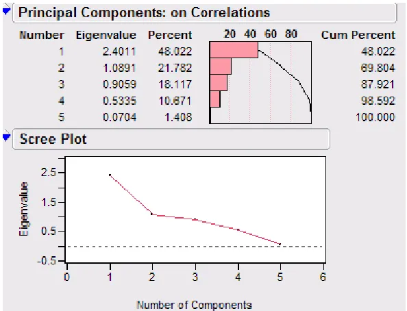
This dimension reduction process was done on several different datasets. PCA was first used on data from the card sliver that was measured on the AFIS (Advanced Fiber Information System) machine. By using
information from the eigenvalue-1 criterion and the scree plot below, the five tested variables were reduced to two principal components that accounted for nearly 70% of the variation. By considering a chart of the
component loadings and variables (see Appendix H), the first component was identified as “particle defects” made up of dust, trash, and VFM (Visible Foreign Matter) variables. The second component was made up of
33
Figure 4.2 Eigenvalue Results and Scree Plot for AFIS Card Sliver Data
PCA was also done on final yarn testing data. The yarn is tested for evenness and imperfections on the Uster testing machine, and four parameters are tested at various levels for a total of twelve different testing
variables. The parameters of interest are CV (coefficient of variation), thin and thick places, and neps which are clusters of fibers in the yarn. The twelve tested variables were highly correlated, and the principal component
analysis showed that two components accounted for 77% of the variation of the original twelve variables. From the scree plot below, there is a clear break in the graph at three components indicating that the two components
above this break were the most significant. These two components could be used in future analyses rather than the original twelve variables. See Appendix I for the rotated factor pattern detailing the component