www.scienceworldjournal.org
ISSN 1597-6343
A Comparative Study of Some Robust Ridge and Liu Estimators
A COMPARATIVE STUDY OF SOME ROBUST RIDGE AND LIU
ESTIMATORS
1Ajiboye S. Adegoke 2Emmanuel Adewuyi 2Kayode Ayinde, and 2Adewale F. Lukman
1Department of Statistics, Federal University of Technology, Akure
2Department of Statistics, Ladoke Akintola University of Technology, P.M.B. 4000, Ogbomoso, Oyo State, Nigeria.
E-Mail: [email protected] , [email protected] , [email protected] , [email protected]
ABSTRACT
In multiple linear regression analysis, multicollinearity and outliers are two main problems. When multicollinearity exists, biased estimation techniques such as Ridge and Liu Estimators are preferable to Ordinary Least Square. On the other hand, when outliers exist in the data, robust estimators like M, MM, LTS and S Estimators, are preferred. To handle these two problems jointly, the study combines the Ridge and Liu Estimators with Robust Estimators to provide Robust Ridge and Robust Liu estimators respectively. The Mean Square Error (MSE) criterion was used to compare the performance of the estimators. Application to the proposed estimators to three (3) real life data set with multicollinearity and outliers problems reveals that the M-Liu and LTS-Liu Estimator are generally most efficient..
Keywords: Ordinary Least Squares, Ridge Regression Estimator, Liu Estimator, Robust Estimator, Robust Ridge Regression Estimator, Robust Liu Estimator
1.0. INTRODUCTION
Regression analysis is used to study the relationship between a single variable Y, called the response variable, and one or more explanatory variable(s),
X
1,
,
X
pby a linear model. Themethod of Ordinary Least Squares (OLS) estimator of model parameters is best linear unbiased estimator (BLUE) and most efficient under certain assumptions (Gujarati, 2003).
One of the assumptions of Linear Regression model is that of independence between the explanatory variables (i.e. no multicollinearity). Violation of this assumption arises most often in regression analysis. Among methods used in detecting the presence of Multicollinearity is variance inflation factor (VIF). The performance of OLS estimator is inefficient if this assumption is not valid and the regression coefficients have large standard errors and sometimes have wrong sign (Gujarati, 2003). In this situation, many estimators have been proposed to combat this problem among which are: Stein Estimator by Stein (1956), Liu Estimator by Liu (1993) and Ridge Estimator proposed by Hoerl and Kennard (1970).
Other problems in regression analysis include the problem of outlier and leverage points. An outlier is an observation that is distant from other observations. Leverage points are points that appear to be outlying in the regressors. Methods such as studentized deleted residual and Mahalanobis distance are used to detect the presence of outliers and leverage point respectively. Cooks D and DFFITS are often used to determine if either the outliers or leverage points influences the regression coefficients. Robust regression estimator is commonly used to circumvent the
problem of outlier. Examples of these estimators are M-estimator proposed by Huber (1964), Least Trimmed Mean (LTS) by Rousseeuw and Van Driessen (1998), S estimator proposed by Rousseeuw and Yohai (1984) and MM estimator by Yohai (1987) among others.
These two problems may jointly exist in regression analysis. This has attracted the attention of some researchers. Holland (1973) proposed robust M-estimator for ridge regression to handle the problem of multicollinearity and outliers. Askin and Montgomery (1980) proposed ridge regression based on the M-estimator. Walker (1984) modified Askin and Montgomery’s approach to allow the use of Generalized M estimators instead of M estimators. Simpson and Montgomery (1996) proposed a biased-robust estimator that uses a multistage Generalized M estimator with fully iterated ridge regression. Lukman et al. (2014) proposed and applied some Robust Ridge Regression Estimators to the Hussein and Abdalla (2012) data. Alpu and Samkar (2010) applied Liu estimator based on M estimator to a VO2 data. The aim of this study is to combine Ridge and Liu estimators with some robust estimators to jointly handle the problem of Multicollinearity and outliers. Also, to compare the performances of these combined estimators with their individual counterparts
2.0. MATERIALS AND METHOD
2.1. Ordinary Least Square Estimator
Consider the standard regression model:
Y
X
(1)where
X
is ann
p
matrix with full rank,Y
is an
1
vector of dependent variable, β is a
p
1
vector of unknown parameters, and
is the error term such thatE
( )
0
and2
(
')
E
I
.Provided
X X
'
is invertible, the OLS estimator is given by1
ˆ ( ' )
X X
X y
'
(2)
The regression model in equation (1) can be written in canonical form
y
Z
(3)Fu
ll L
en
gt
h Rese
ar
ch
Ar
A Comparative Study of Some Robust Ridge and Liu Estimators
where
Z
XQ
,
Q
'
and Q is the orthogonal matrix with columns that constitute the eigenvectors ofX X
'
. Then1 2
'
'
'
( ,
,...,
p)
Z Z
Q X XQ
diag
,where
1
2
...
p are ordered eigenvalues of X’X.Thus, the Ordinary Least Square Estimator of α is
1
ˆ
OLSZ y
'
(4)2.2. Ridge RegressionEstimator
If 𝑍′𝑍 matrix is ill-conditioned, (especially when there is a near-linear dependency among the explanatory variables), the OLS
estimator of
tends to havea large variance. Ridge parameter is added to the 𝑍′𝑍 matrix to reduce the collinearity effect. Hoerl and Kennard (1970) defined the ridge regression estimator of
as:𝛼̂(𝑘) = (𝑍′𝑍 +
𝑘𝐼)−1𝑍′𝑦 (5) where k is the ridge parameter. The value of k used in this study is the one proposed by Lukman (2015).
2 2
1
ˆ
ˆ
max(
)
ALi
K
(6)where 𝜎̂2 is the estimated MSE calculated as 𝜎̂2=∑𝑛𝑖=1𝑒𝑖2
𝑛−𝑝 and
𝛼̂ is the estimated regression coefficient.
2.3. Liu Estimator
To overcome multicollinearity, Liu (1993) proposed the Liu Estimator by combining the Stein estimator with Ridge estimator to form
1
ˆ
(
'
) (
'
)
ˆ
LX X
I
X X
dI
OLS
(7) where d is the Biasing parameter and can be computed according to Liu by
1 2
2
2 1
1
(
1)
ˆ
1
ˆ
(
1)
p
i i i
L p
i
i i
d
(8) where
ˆ
Q
'
ˆ
OLS and
ˆ
2 are Ordinary Least Squareestimators of α and
2 respectively, and Q is the matrix ofeigenvectors corresponding to the eigenvalues o the matrix X’X. Now equation (7) can be written in canonical form:
1
ˆ
L(
I
p) (
d I
L p)
ˆ
OLS
(9) where IP is the p-identity matrix
2.4. Robust Regression
2.4.1. M-Estimator
The most common method of robust regression is M-estimation, introduced by Huber (1964). It is nearly as efficient as OLS. Rather than minimizing the sum of squared errors, M-estimate chooses 𝛽 to minimize
∑ 𝜌 (𝑦𝑖−𝑥𝑖𝑇𝛽̂
𝜎 )
𝑛
𝑖=1 (10)
Possible choices of 𝜌 are:
𝜌(𝑥) = 𝑥2 is just least squares and 𝜌(𝑥) = |𝑥| is called the least absolute deviations regression (LAD).
𝜌(𝑥) =
{ 𝑥2
2, 𝑖𝑓 |𝑥| ≤ 𝑐 ⁄
𝑐|𝑥| −𝑐2
2, 𝑜𝑡ℎ𝑒𝑟𝑤𝑖𝑠𝑒
(11)
Differentiating the M-estimate criterion with respect to 𝛽𝑗and setting to zero, we get;
∑ 𝜌 (𝑦𝑖−∑ 𝑥𝑖𝑗𝛽𝑗 𝑝 𝑗=1
𝜎 )
𝑛
𝑖=1 𝑥𝑖𝑗= 0, 𝑗 =
1, … , 𝑝 (12)
Now let 𝑢𝑖= 𝑦𝑖− ∑𝑝𝑗=1𝑥𝑖𝑗𝛽𝑗 to get
∑ 𝜌′(𝑢𝑖)
𝑢𝑖 𝑥𝑖𝑗(𝑦𝑖− ∑ 𝑥𝑖𝑗𝛽𝑗
𝑝
𝑗=1 )
𝑛
𝑖=1 =
0 (13) making the identification of
𝑤(𝑢) =𝜌′𝑢(𝑢)and find 𝑤(𝑢) for choices of 𝜌 above:
1. LS: 𝑤(𝑢)is constant.
2. LAD: 𝑤(𝑢) = 1/|𝑢|
3. Huber: 𝑤(𝑢) = {1, 𝑖𝑓 |𝑢| ≤ 𝑐𝑐 |𝑢|, 𝑜𝑡ℎ𝑟𝑤𝑖𝑠𝑒
2.4.2. MM-Estimator
It was first introduced by Yohai (1987). It has become increasingly popular and perhaps one of the most commonly employed robust regression technique. The ‘‘MM’’ in the name refers to the fact that more than one M-estimation procedure is used to calculate the final estimates. Following from the M-estimation case, iteratively reweighted least squares (IRLS) is employed to find estimates. The procedure is as follows:
1. Initial estimates of the coefficients 𝛽̂(1) and corresponding residuals 𝑒𝑖(1) are taken from a highly resistant regression (i.e., a regression with a breakdown point of 50%). Although the estimator must be consistent, it is not necessary that it be efficient. As a result, S-estimation with Huber or bisquare weights (which can be seen as a form of M-estimation) is typically employed at this stage.
2. The residuals 𝑒𝑖(1)from the initial estimation at Stage 1 are used to compute an M-estimation of the scale of the residuals,
𝜎̂𝑒.
3. The initial estimates of the residuals from Stage 1 and of the residual scale 𝜎̂𝑒 from Stage 2 are used in the first iteration of weighted least squares to determine the M-estimates of the regression coefficients
∑ 𝑤𝑖(𝑒𝑖 (1)
/𝜎̂𝑒) 𝑥𝑖 = 𝑛
𝑖=1
0
(14)
where the 𝑤𝑖 are typically Huber or bisquare weights.
4. New weights are calculated, 𝑤𝑖(1), using the residuals from the initial WLS (Step 3).
5. Keeping constant the measure of the scale of the residuals from Step 2, Steps 3 and 4 are continually reiterated until convergence.
A Comparative Study of Some Robust Ridge and Liu Estimators 2.4.3. S-Estimator
In response to the low breakdown point of M-estimators. Rousseeuw and Yohai (1984) proposed S-estimates by considering the scale of the residuals. S-estimates are the solution that finds the smallest possible dispersion of the residuals
𝑚𝑖𝑛𝜎̂ (𝑒𝑖(𝛽̂), … , 𝑒𝑛(𝛽̂)). Rather than minimizing the variance of the residuals, robust S-estimation minimizes a robust M-estimate of the residual scale
1
𝑛∑ 𝜌 (
𝑒𝑖
𝜎 ̂𝑒)
𝑛
𝑖=1 = 𝑏, (15)
where b is a constant defined as 𝑏 = 𝐸𝜙[𝜌(𝑒)]and 𝜙 represents the standard normal distribution. Differentiating Equation 18 and solving results in
1
𝑛∑ 𝜓 (
𝑒𝑖
𝜎 ̂𝑒) ,
𝑛
𝑖=1 (16)
where 𝜓 is replaced with an appropriate weight function. As with most M-estimation procedures, either the Huber weight function or the biweight function is usually employed.
2.4.4. Least Trimmed Squares (LTS) Estimator
Another method developed by Rousseeuw (1998) is least trimmed squares (LTS) regression. Extending from the trimmed mean, LTS regression minimizes the sum of the trimmed squared residuals. The LTS estimator is found by;
𝑚𝑖𝑛 ∑ 𝑒(𝑖)2, 𝑞
𝑖=1
where 𝑞 = [𝑛(1 − 𝛼) + 1] is the number of observations included in the calculation of the estimator, and α is the proportion of trimming that is performed. Using 𝑞 = (𝑛
2) + 1 ensures that the estimator has a breakdownpoint of 50%.
2.5. Robust Ridge Regression (RRR)
To solve the problems of multicollinearity and outlier simultaneously, the ridge estimator was combined with some robust estimators (M, MM, LTS and S estimators) to form robust ridge estimator (RRE) which are M-Ridge, MM-Ridge, LTS-Ridge and S-Ridge estimators (Lukman et al., 2014). These Robust ridge estimators can be computed as:
𝛼̂𝑅𝑅= (𝑍′𝑍 + 𝑘𝐴𝐿𝑟𝑜𝑏𝑢𝑠𝑡𝐼𝑝) −1
𝑍′𝑌 (17)
where 𝑘𝐴𝐿𝑟𝑜𝑏𝑢𝑠𝑡 is the robust ridge parameter. It is obtained from the robust regression methods instead of the OLS estimation, and can be computed as given below;
2
1
ˆ
ˆ
max(
)
ALrobust
Robust Robust
k
2.6. Robust Liu Estimator (Proposed)
To solve the problems of multicollinearity and outlier simultaneously, Liu estimator combined with some robust estimators (M, MM, LTS and S estimators) to provide robust Liu
estimator (RLE) which are M-Liu, MM-Liu, LTS-Liu and S-Liu estimators. These Robust Liu estimators can be computed as:
1
ˆ
RLE(
I
p) (
d I
R p)
ˆ
R
(19)
where
d
R is the biasing parameter obtained from robust estimators, computed as:1 2
2 2 1
1
(
1)
ˆ
1
ˆ
(
1)
pi i i R Robust p
iRobust i i
d
(20)
2.7. Data Description
Three datasets are used in this study to examine the performance of the estimators. The datasets are given in details below.
2.7.1. Longley Data
Longley Data is a macroeconomic dataset which provides a well-known example for a highly collinear regression. A data frame with seven economic variables observed yearly from 1947 to 1962. The variables are: Employment, Prices, Unemployed, Military, GNP, Population Size, Year. GNP is the Gross National Product, Employment is the number of people employed, Unemployed is the number of unemployed, Military is the number of people in the armed forces, Population size is the non-institutionalized population of persons at age ≥14 years, Price is the GNP implicit price deflator and year is the time.
Longley data have been diagnosed to suffer both problems of multicollinearity and outlier (Cook, 1977; Besley et al., 1980; and Jahufer, 2013).
2.7.2. Portland cement data
Portland dataset traceable to Woods et al. (1932) has been widely analysed by Kaciranlar et al. (1999). The dataset contains four explanatory varaiables which are tricalcium aluminate (X1),
tricalcium silicate (X2), tetracalcium aluminoferrite (X3) and
β-dicalcium silicate (X4). The heat evolved after 180 days of curing
is the dependent variable (Y). The dataset suffers multicollinearity since variance inflation factors are greater than 10. Mahalanobis distances of observations 3 and 10 revealed that the observations are leverage. With this it is obvious that there is outlier in the x-direction and no outlier in the y-x-direction. As a result, it is observed that multicollinearity and leverage point exists jointly in the dataset.
2.7.3. Hussein and Abdalla data
This dataset was used by Hussein and Abdalla (2012) and it covered the products in the manufacturing sector of Iraq in the period of 1960 to 1990. The variables used are the product value in the manufacturing sector(Y), value of imported intermediate (X1), imported capital commodities (X2) and value of imported raw
materials (X3). Hussein and Abdalla (2012) showed that the
dataset suffers the problem of multicollinearity since VIF > 10. Lukman et al. (2014) identified case number: 12, 14, 15, 16, 17, 18, 19, 20 and 21 as outliers in the y-direction and also identified case number 12, 14 and 15 as leverages. Therefore, outliers exist in the y and x direction.
A Comparative Study of Some Robust Ridge and Liu Estimators 2.8. Criterion for investigation
To investigate whether the robust ridge estimator is better than the OLS estimator, the MSE was calculated as follows:
𝑀𝑆𝐸(𝛼̂ 𝑅𝑖𝑑𝑔𝑒) = 𝜎̂𝑂𝐿𝑆2 ∑ 𝜆𝑖
(𝜆𝑖+𝑘𝑂𝐿𝑆)2+
𝑝 𝑖=1
𝑘𝑂𝐿𝑆∑
𝛼𝑖,𝑂𝐿𝑆2
(𝜆𝑖+𝑘𝑂𝐿𝑆)2
𝑝
𝑖=1 (20)
𝑀𝑆𝐸(𝛼̂𝑅𝑜𝑏𝑢𝑠𝑡 𝑅𝑖𝑑𝑔𝑒) = 𝜎̂𝑟𝑜𝑏𝑢𝑠𝑡2 ∑ 𝜆𝑖
(𝜆𝑖+𝑘𝑅)2+
𝑝 𝑖=1
𝑘𝑅2∑
𝛼𝑖,𝑟𝑜𝑏𝑢𝑠𝑡2
(𝜆𝑖+𝑘𝑅)2
𝑝
𝑖=1 (21)
𝑀𝑆𝐸(𝛼̂𝐿𝑖𝑢) = 𝜎̂2∑
(⋋𝑖+𝑑)2
(⋋𝑖+1)2
𝑃
𝑖=1 + (𝑑 −
1)2∑ 𝛼̂𝑖2
(⋋𝑖+1)2
𝑃
𝑖=1 (22)
𝑀𝑆𝐸(𝛼̂ 𝑅𝑜𝑏𝑢𝑠𝑡 𝐿𝑖𝑢) = 𝜎̂𝑟𝑜𝑏𝑢𝑠𝑡2 ∑
(⋋𝑖+𝑑𝑅)2
(⋋𝑖+1)2
𝑃
𝑖=1 + (𝑑𝑅−
1)2∑ 𝛼̂𝑖,𝑟𝑜𝑏𝑢𝑠𝑡2
(⋋𝑖+1)2
𝑃
𝑖=1 (23)
𝑀𝑆𝐸(𝛼̂𝑂𝐿𝑆) =
𝜎̂2∑ 1 𝜆𝑖
𝑝
𝑖=1 (24)
where 𝜆𝑖, (𝑖 = 1,2, … , 𝑝) are the eigenvalues of 𝑋′𝑋, k is the ridge parameter obtained from OLS and Robust estimates,
𝛼𝑖 (𝑖 = 1,2, … , 𝑝) is the ith element of the vector 𝛼 = 𝑄′𝛽.
3.0. RESULTS AND DISCUSSION
3.1. Result for Longley Data
Table 1: Summary of OLS and Robust Estimates
Table 2: Summary of the Influential and Leverage Points
Table 3: Estimates of Ridge, Liu, Robust Ridge and Robust Liu Estimators
From Table 1, it is obvious that the data suffers a severe problem of multicollinearity since the Variance Inflation Factors (VIF) are greater than 10 except for X5. Also from Table 2, the data has
outliers in the y-direction, hence the data suffers both problem of multicollinearity and outliers. It follows from Table 3 that the two problems have been circumvented with the use of Robust Liu and Robust Ridge Regression Estimators and it is found that the Robust Liu is the most efficient in term of MSE.
3.2. Results for Portland Cement Data Table 4: Estimates of OLS and Robust estimators
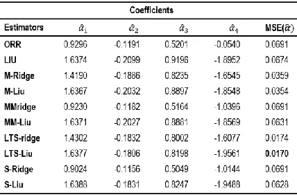
Table 5: Estimates of Ridge, Liu, Robust Ridge and Robust Liu estimators
From Table 4 and 5, it can be seen that in terms of MSE criterion of the estimators, the LTS-Liu, LTS-Ridge in this order, are more efficient than the OLS. Thus, LTS-Liu is most efficient.
3.3. Result for Hussein and Abdalla Data
Table 6: Estimates of OLS and Robust estimator
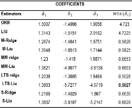
A Comparative Study of Some Robust Ridge and Liu Estimators Table 7: Estimates of Ridge, Liu, Robust Ridge and Robust Liu
estimators
The result in Table 7 shows that robust Liu (LTS-Liu) and robust Ridge (LTS-Ridge) regression estimators have least mean square error.
4.0. Conclusion
Ordinary Least Square (OLS), Liu Regression and Ordinary Ridge Regression (ORR) estimators could not perform well in term of their Mean Squared Error (MSE) in the presence of multicollinearity and outlier but ORR and Liu estimator performs better than that of Ordinary Least Square (OLS) Estimator. It is observed that Robust Ridge Estimators (RRE) and Robust Liu estimators perform better than the ORR, LRE and OLS estimators when both problems exist. Finally, M-Liu and M-Ridge perform most in this order when the outliers are in y-direction, while LTS-Ridge and LTS-Liu perform better when the outliers are in x-direction (Leverage).
REFERENCES
Alpu, O. and Samkar, H. (2010). Liu Estimator based on an M Estimator. Turkiye Klinikleri
Biostat, 2(2):49-53.
Askin, G. R., and Montgomery, D. C. (1980). Augmented robust estimators. Techonometrics,
22, 333-341.
Chatterjee, S. and Hadi, A. S. (1988). Sensitivity Analysis in Linear Regression. Wiley Series
in Probability and Mathematical Statistics.Wiley, New York.
Cook, R.D. (1977). Detection of influential observations in linear regression. Technometrics,
19, 15-18.
Belsley, D. A, Kuh, E. and Welsch, R. E. (1980). Regression Diagnotics: Identifying
Influence Data and Source of Collinearity. Wiley, New York.
Gujarati, N. D. (2003). Basic Econometrics, New Delhi: Tata McGraw-Hill, New York.
Hoerl, A. E. and Kennard, R.W. (1970). Ridge Regression Biased Estimation for
Nonorthogonal Problems.Technometrics,12, 55-67.
Holland, P. W. (1973). Weighted ridge regression: Combining ridge and robust regression
methods. NBER Working Paper Series, 11, 1-19. Huber, P.H. (1964). Robust estimation of a location parameter.
The Annals of Mathematical Statistics, 35, 101. Hussein, Y. A. and Abdalla, A. A. (2012). Generalized Two stages
Ridge Regression Estimator for Multicollinearity and Autocorrelated errors. Canadian Journal on Science and Engineering Mathematics, 3(3), 79-85.
Jahufer, A. (2013). Detecting Global Influential Observations in Liu Regression Model. Open
Journal of Statistics, 3, 5-11.
Kaciranlar, S., Sakallioglu, S., Akdeniz, F., Styan., G. P. H., and Werner, H. J. (1999). A new biased estimator in linear regression and a detailed analysis of the widely-analysed dataset on portland cement. Sankhya, Ser. B, Indian J.Statist., 61: 443-459.
Liu, K. (1993). A new class of biased estimate in linear regression. Communication
in Statistics. 22(2):393-402.
Longley, J. W. (1967). An Appraisal of Least Squares Programs for Electronic Computer
for the Point of View of the User. Journal of American Statistical Association.
62(319), 819-841.
Lukman, A. F, Arowolo, O. and Ayinde, K. (2014). Some Robust Ridge Regession for Handling Multicollinearity and Outliers. International Journal of Sciences: Basic and Applied Research (IJSBAR). 16(2), 192-202. Lukman, A. F. (2015). Review and Classifications of the Ridge
Parameter Estimation Techniques.
UnpublishedM.phil./ PhD thesis.
Rousseeuw, P.J. and Van Driessen, K. (1998). Computing LTS Regression for Large Data Sets, Technical Report, University of Antwerp, submitted.
Rousseeuw, P.J., and Yohai. (1984). Robust regression by means of S estimators. In W. H. J. Franke and D.Martin, Robust and Nonlinear Time Series Analysis, Springer-Verlag, New-York, 256-272.
Simpson, J. R., and Montgomery, D. C. (1996). A biased robust regression technique for combined outlier-multicollinearity problem. Journal of Statistical Computation Simulation, 56, 1-22.
Stein, C. (1956). Inadmissibility of the usual estimator for the mean of a multivariate normal distribution. In Proceedings of the Third Berkeley symposium on mathematical statistics and probability, 1, 197– 206. Walker, E. (1984). Influence, collinearity and robust estimation in
regression. Unpublished Ph.D. dissertation, Department of Statistics, Virginia Polytechnic Institute. Woods, H, Steinour, H. and Starke, H. (1932). Effect of
Composition of Portland
Cement on Heat Evolved During Hardening, Industrial and Engineering Chemistry,
24, 1207-1214.
Yohai, V.J. (1987). High breakdown point and high breakdown-point and high efficiency robust estimates for regression. The Annals of Statistics, 15, 642-656.