UDLAP at SemEval-2016 Task 4: Sentiment Quantification Using a Graph
Based Representation
Esteban Castillo1, Ofelia Cervantes1, Darnes Vilari˜no2 and David B´aez1
1Universidad de las Am´ericas Puebla
Department of Computer Science, Electronics and Mechatronics, Mexico
{esteban.castillojz, ofelia.cervantes, david.baez}@udlap.mx
2Benem´erita Universidad Aut´onoma de Puebla
Faculty of Computer Science, Mexico
Abstract
We present an approach for tackling the tweet quantification problem in SemEval 2016. The approach is based on the creation of a co-occurrence graph per sentiment from the train-ing dataset and a graph per topic from the test dataset with the aim of comparing each topic graph against the sentiment graphs and eval-uate the similarity between them. A heuristic is applied on those similarities to calculate the percentage of positive and negative texts. The overall result obtained for the test dataset ac-cording to the proposed task score (KL diver-gence) is0.261, showing that the graph based representation and heuristic could be a way of quantifying the percentage of tweets that are positive and negative in a given set of texts about a topic.
1 Introduction
In the past decade, new forms of communication, such as microblogging and text messaging have emerged and become ubiquitous. There is no limit to the range of information conveyed by tweets and texts. These short messages are extensively used
toshare opinions and sentimentsthat people have
about their topics of interest. Working with these informal text genres presents challenges for Natural Language Processing (NLP) beyond those encoun-tered when working with more traditional text gen-res. Typically, this kind of texts are short and the language used is very informal. We can find cre-ative spelling and punctuation, slang, new words, URLs, and genre-specific terminology and
abbrevi-ations that make their manipulation more challeng-ing.
Representing that kind of text for automatically mining and understanding the opinions and senti-ments that people communicate inside them has very recently become an attractive research topic (Pang and Lee, 2008). In this sense, the experiments re-ported in this paper were carried out in the frame-work of the SemEval 20161 (SemanticEvaluation) which has created a series of tasks for sentiment analysis on Twitter (Nakov et al., 2016b). Among the proposed tasks we chose Task 4, subtask D which was namedtweet quantification according
to a two-point scale and was defined as follows:
”Given a set of tweets known to be about a given topic, estimate the distribution of the tweets across the Positive and Negative classes”. In order to solve this task we created an algorithm that builds up graphs to compare each topic against all possible sentiments for obtaining the polarity percentage of each one. The steps involved in our sentiment quan-tification process are then discussed in detail.
The rest of the paper is structured as follows: in Section 2 we present some related work found in the literature with respect to the quantification of senti-ments in text docusenti-ments. In Sections 3 to 5 the algo-rithm and the graph representation used to detect the percentage of texts for each sentiment are explained. In Section 6, the experimental results are presented and discussed. Finally, in Section 7 the conclusions as well as further work are described.
1http://alt.qcri.org/semeval2016/
Algorithm 1Sentiment quantification process
Input:
/*Preprocess documents*/
X ={x1, ..., xm}positive training docs.
Y ={y1, ..., yn}negative training docs.
Z ={z1, ..., zs}topic names
DT ={DT[z1], ..., DT[zs]}test docs per topic.
Output:
/* Positive (p) and negative (n) polarity
percentage for each topic*/
P T ={(p1, n1), ...,(ps, ns)}
Procedure:
/* LetGP ositiveandGN egativedenote the graphs
of the positive an negative documents created fromXandY*/
GP ositive,GN egative
foreachziinZdo
/*LetGT opicdenote a topic graph
created fromDT[zi]*/
GT opic
/*Similarity between topic and sentiments, see algorithm 2*/
Sim1 =Similarity(GT opic, GP ositive)
Sim2 =Similarity(GT opic, GN egative)
/*Apply a heuristic*/
ifSim1 > Sim2then
P T[zi] = (1−Sim1, Sim1)
else
P T[zi] = (Sim2,1−Sim2)
end if end for
2 Related Work
There exist a number of works in literature associ-ated to the automatic quantification of sentiments in documents. Some of these works have focused on the contribution of particular features, such as the use of the vocabulary to extract lexical elements as-sociated to the documents (Kim and Hovy, 2006), the use of part-of-speech tag n-grams and syntactic phrase patterns (Esuli et al., 2010) to capture syn-tactic features of texts associated with a sentiment, the use of dictionaries and emoticons of positive and negative words (Go et al., 2009) as well as
man-ually and semiautomatically constructed syntactic and semantic phrase and lexicons (Gao and Sebas-tiani, 2015; Whitelaw et al., 2005).
On the other hand, many contributions focused on the use of structures to represent the features associ-ated to a document like the frequency of occurrence vector (Manning et al., 2008; Balinsky et al., 2011) or the vectors that represent the presence or absence of features (Kiritchenko et al., 2014). But research works that use graph representations for texts in the context of sentiment quantification barely appear in the literature (Pinto et al., 2014; Poria et al., 2014). It has usually been proposed the concept of n-grams with a frequency of occurrence vector to solve it (Pang and Lee, 2008). However, there is still an enormous gap between this approach and the use of more detailed graph structures that represent in a natural way the lexical, semantic and stylistic fea-tures.
3 Sentiment Quantification
Algorithm 1 shows the steps involved in computing the percentage of positive and negative tweets for each topic in the test dataset (see section 6.1) con-sidering the use of graphs to represent the word in-teraction for each sentiment in the training dataset and for each topic in the test dataset. The algorithm consists of five relevant stages:
1. Preprocess all documents in the dataset. This task includes elimination of punctuation sym-bols and all the elements that are not part of the ASCII encoding. Then, all the remaining words are changed to lowercase.
2. Create a graph for each sentiment using the
trainingdataset documents (see Section 4).
3. Create a graph for each topic using the test
dataset documents (see Section 4).
4. Compare each topic graph against the senti-ment graphs and calculate the similarity score between both (see Section 5).
that the sum of all percentages related to a topic must be equal to one2.
4 Graph Based Representation
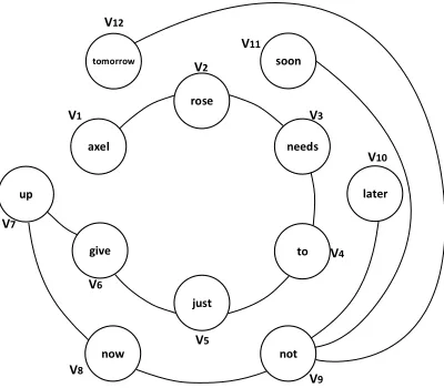
Among different proposals for mapping texts to graphs, the co-occurrence of words (Sonawane and Kulkarni, 2014; Balinsky et al., 2011) has become a simple but effective way to represent the relation-ship of one term over another one in texts where there is no syntactic order (usually social media texts like Twitter or SMS). Formally, the proposed co-occurrence graph used in the experiments is repre-sented byG= (V, E), where:
• V ={v1, ..., vn}is a finite set ofverticesthat
consists of the words contained in one or sev-eral texts.
• E⊆V×V is the finite set ofedgeswhich
rep-resent that two vertices are connected if their corresponding lexical unitsco-occur within a
window of maximum 2 words in the text (at
least once). We consider this type of window because it represents the natural relationship of words.
As an example, consider the following sentenceζ
extracted from a text T in the dataset: “Axel Rose
needs to just give up. Now. Not later, not soon, not tomorrow.”, which after the preprocessing stage (see Section 3) would be as follows: “axel rose needs to just give up now not later not soon not tomorrow”. Based on the proposed representation, preprocessed sentenceζ can be mapped to the
co-occurrence graph shown in Figure 1.
5 Graph similarity
After having created the graph representation for each topic and sentiment in the dataset, the steps in-volved in computing the similarity score (Castillo et al., 2015) are shown in algorithm 2. The algorithm consists of four relevant stages:
1. Obtain all vertices (words) that share the topic graph as well as the sentiment graph.
2. Apply the Dice similarity measure (Montes et al., 2000; Adamic and Adar, 2003) for each
2SemEval 2016 task 4, subtask D requirement.
axel
rose
needs
to
just give
tomorrow soon
later
not now
up V1
V2
V3
V4
V6
V12
V11
V10
V9
V7
V8
[image:3.612.327.527.61.236.2]V5
Figure 1: co-occurrence graph example.
graph, taking as input the shared vertices of the previous step and the graph to be analyzed. The result is a matrix that represents the similarity scores for each pair of input vertices, based on their connection patterns. Formally, Dice sim-ilarity calculates the simsim-ilarity of two vertices (x, y) as twice the number of common
neigh-bors (ngb) divided by the sum of the neighbors
of the vertices (see equation 1).
Dice(x, y) = 2|ngb(x)∩ngb(y)|
|ngb(x)|+|ngb(y)| (1)
3. Obtain the upper triangular values for each ma-trix and use them to build a vector represen-tation (Manning et al., 2008). The rest of the matrix values are not useful, because the main diagonal represents the similarity of an input vertex with itself and the lower triangular is the same as the upper one.
4. Apply the normalized Euclidean distance (Can-cho, 2004) between the vector representing the topic and the vector representing a sentiment. The result is a value in the range of0to1that
indicates how similar the two graphs are. The Euclidean distance of vectorAandB is
calcu-lated using equation 2.
Euclidean(A, B) =
v u u tXn
i=1
(Ai−Bi)2
Algorithm 2Similarity between graphs
functionSimilarity(GA, GB)
/* LetV(GA)denote the set of vertices
of graphGA*/
V(GA)
/* LetV(GB)denote the set of vertices
of graphGB*/
V(GB)
/* Calculate the Intersection between graphsGAandGB*/
I =V(GA)∩V(GB)
/* Apply Dice similarity for each pair of shared vertices in both graphs, see equation 1*/
ResultM atrixA=DiceSim(GA, I)
ResultM atrixB =DiceSim(GB, I)
/* LetV ectorAdenote the upper
triangular values ofResultM atrixA*/
V ectorA
/* LetV ectorBdenote the upper
/* triangular values ofResultM atrixB*/
V ectorB
/* Apply the normalized Euclidean distance taking as input both vectors, see equation 2*/
Result = Euclidean(V ectorA, V ectorB)
returnResult
end function
6 Experimental results
The results obtained with the proposed approach are discussed in this section. First, we describe the dataset used in the experiments and, thereafter, the results obtained.
6.1 Dataset
The document collection used in the experiments is a subset of the SemEval 2016 task 4 corpus (Nakov et al., 2016b), which includes, several text docu-ments in English on different topics and genres. The dataset is divided in two groups:
• Training documents:It contains a set of topics
each one with a set of known documents. For each document a label that indicates the polar-ity of the text (positive or negative) is assigned.
• Test documents: It contains a set of topics3
[image:4.612.318.538.214.315.2]each one with a set of known documents. In this case there is no label that indicates the po-larity of the text. These documents are used to test our algorithm taking into account the writ-ing style samples of the trainwrit-ing documents. In Table 1, main dataset features are shown, in-cluding the number of documents per topic for the training and test dataset.
Table 1: SemEval task 4 subtask D dataset features.
Feature Training Test
Type of documents Tweet Tweet Number of documents 5205 10551
Number of topics 59 100
Number of documents per topic 70-100 60-250 Avg. words per document 68 52 Avg. words per sentence 5 5
Vocabulary size 6869 9732
6.2 Obtained results
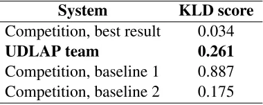
In Table 2 we present results obtained with the test dataset considered in the SemEval 2016 task 4 sub-task D. The results were evaluated according to the Kullback-Leibler Divergence (KLD), which is a measure of the error made in estimating a true dis-tribution p over a set C of classes by means of a
predicted distributionpˆ. KLD (Nakov et al., 2016a)
is a measure of error, so lower values are better (see equation 3).
KLD(ˆp, p, C) = X cj∈C
p(cj)log
p(cj) ˆ
p(cj) (3)
Table 2: Evaluation of the proposed algorithm using the test dataset.
System KLD score
Competition, best result 0.034
UDLAP team 0.261
Competition, baseline 1 0.887 Competition, baseline 2 0.175
Taking into account obtained results, our ap-proach performed above the baseline 1 and slightly
[image:4.612.319.509.577.653.2]below baseline 2. We consider that these results were obtained even though the training corpus was very unbalanced (there were more positive texts than others) and there was a high difference between the vocabulary of the topics of the training and test datasets. The proposed algorithm showed an effec-tive and relaeffec-tive fast way4(00:02:48 minutes) to get the percentage of positive and negative documents although it is necessary to perform different experi-ments using the proposed approach on a test dataset with more topics. Further analysis on the use of a co-occurrence graph and the similarity measure will allow us to find more accurate features that can be used for the sentiment quantification problem.
7 Conclusions
We have presented an approach that incorporates the use of a graph representation to solve the sentiment quantification problem (task 4 subtask D). The re-sults obtained show a competitive performance that is above one of the baseline scores. However there is still a great challenge to improve the techniques for dealing with the quantification problem where the text could be smaller and there are different topics, each one with his own vocabulary. One of the con-tributions of this paper is that we proposed a graph based representation and a similarity measure for the quantification problem instead of using traditional classification techniques like a supervised learning method based on the extraction of stylistic features (Kharde and Sonawane, 2016). As further work we propose the following:
• Use different co-occurrence windows for mod-eling the text using a graph based representa-tion.
• Experiment with other graph representations for texts that include alternative levels of lan-guage descriptions such as the use of sen-tence chunks, pragmatic sensen-tences, etc (Mihal-cea and Radev, 2011).
• Propose a similarity measure that uses the se-mantic information of a graph (Alvarez and Yan, 2011).
4The execution runtime consider all the steps involved in algorithm 1.
• Explore different techniques that can be used in the sentiment quantification problem (Pang and Lee, 2008).
• Compare the algorithm presented with other
classical approaches like the use of stylistic fea-tures or the N-gram model (Stamatatos, 2008).
• Explore different supervised/unsupervised
classification algorithms (Cook and Holder, 2000).
Acknowledgments
This work has been supported by the CONA-CYT grant with reference #373269/244898 and the CONACYT-PROINNOVA project no. 0198881.
References
Lada Adamic and Eytan Adar. 2003. Friends and neigh-bors on the web. Social Networks, 25(3):211–230. Marco Alvarez and Changhui Yan. 2011. A graph-based
semantic similarity measure for the gene ontology. J. Bioinformatics and Computational Biology, 9(6):681– 695.
Helen Balinsky, Alexander Balinsky, and Steven Simske. 2011. Document sentences as a small world. InSMC, pages 2583–2588. IEEE.
Ramon Cancho. 2004. Euclidean distance between syn-tactically linked words.Phys. Rev. E, 70(5), nov. Esteban Castillo, Ofelia Cervantes, Darnes Vilari˜no, and
David B´aez. 2015. Author verification using a graph-based representation. International Journal of Com-puter Applications, 123(14):1–8, August.
Diane Cook and Lawrence Holder. 2000. Graph-based data mining.IEEE Intelligent Systems, 15(2):32–41. Andrea Esuli, Fabrizio Sebastiani, and Ahmed ABBASI.
2010. Sentiment quantification. IEEE intelligent sys-tems, 25(4):72–79.
Wei Gao and Fabrizio Sebastiani. 2015. Tweet senti-ment: From classification to quantification. In Pro-ceedings of the 2015 IEEE/ACM International Con-ference on Advances in Social Networks Analysis and Mining 2015, pages 97–104. ACM.
A Go, L Huang, and R Bhayani. 2009. Sentiment analy-sis of twitter data. Entropy, 2009(June):17.
Vishal Kharde and Sheetal Sonawane. 2016. Senti-ment analysis of twitter data : A survey of techniques.
CoRR.
Svetlana Kiritchenko, Xiaodan Zhu, and Saif Moham-mad. 2014. Sentiment analysis of short informal texts.
J. Artif. Intell. Res. (JAIR), 50:723–762.
Christopher Manning, Prabhakar Raghavan, and Hinrich Sch¨utze. 2008. Introduction to Information Retrieval. Cambridge University Press.
Rada Mihalcea and Dragomir Radev. 2011. Graph-based natural language processing and information retrieval. Cambridge University Press.
Manuel Montes, Aurelio L´opez, and Alexander Gelbukh. 2000. Information retrieval with conceptual graph matching. In Lecture Notes in Computer Science, number 1873, pages 312–321. Springer-Verlag. Preslav Nakov, Alan Ritter, Sara Rosenthal, Fabrizio
Se-bastiani, and Veselin Stoyanov. 2016a. Evaluation measures for the semeval-2016 task 4 sentiment analy-sis in Twitter. InProceedings of the 10th International Workshop on Semantic Evaluation, SemEval ’16, San Diego, California, June. Association for Computa-tional Linguistics.
Preslav Nakov, Alan Ritter, Sara Rosenthal, Veselin Stoy-anov, and Fabrizio Sebastiani. 2016b. SemEval-2016 task 4: Sentiment analysis in Twitter. InProceedings of the 10th International Workshop on Semantic Eval-uation, SemEval ’16, San Diego, California, June. As-sociation for Computational Linguistics.
Bo Pang and Lillian Lee. 2008. Opinion mining and sentiment analysis. Foundations and Trends in Infor-mation Retrieval, 2(1-2):1–135.
David Pinto, Darnes Vilari˜no, Saul Le´on, Miguel Jasso, and Cupertino Lucero. 2014. Buap: Polarity classifi-cation of short texts. InProceedings of the 8th Inter-national Workshop on Semantic Evaluation (SemEval 2014), pages 154–159. Association for Computational Linguistics and Dublin City University, August. Soujanya Poria, Erik Cambria, Gr´egoire Winterstein,
and Guang-Bin Huang. 2014. Sentic patterns: Dependency-based rules for concept-level sentiment analysis. Knowl.-Based Syst., 69:45–63.
S. S. Sonawane and P. A. Kulkarni. 2014. Article: Graph based representation and analysis of text document: A survey of techniques. International Journal of Com-puter Applications, 96(19):1–8, June.
Efstathios Stamatatos. 2008. Author identification: Us-ing text samplUs-ing to handle the class imbalance prob-lem. Inf. Process. Manage., 44(2):790–799, mar. Casey Whitelaw, Navendu Garg, and Shlomo Argamon.