Speeding Up Neural Machine Translation Decoding by Cube Pruning
Wen Zhang1,2 Liang Huang3,4 Yang Feng1,2 Lei Shen1,2 Qun Liu5,1
1Key Laboratory of Intelligent Information Processing
Institute of Computing Technology, Chinese Academy of Sciences (ICT/CAS)
2University of Chinese Academy of Sciences, Beijing, China
{zhangwen,fengyang,shenlei17z}@ict.ac.cn
3Oregon State University, Corvallis, OR, USA 4Baidu Research, Sunnyvale, CA, USA
5Huawei Noah’s Ark Lab, Hong Kong, China
Abstract
Although neural machine translation has achieved promising results, it suffers from slow translation speed. The direct conse-quence is that a trade-off has to be made be-tween translation quality and speed, thus its performance can not come into full play. We apply cube pruning, a popular technique to speed up dynamic programming, into neural machine translation to speed up the transla-tion. To construct the equivalence class, simi-lar target hidden states are combined, leading to less RNN expansion operations on the target side and lesssoftmaxoperations over the large target vocabulary. The experiments show that, at the same or even better translation quality, our method can translate faster compared with naive beam search by3.3×on GPUs and3.5×
on CPUs.
1 Introduction
Neural machine translation (NMT) has shown promising results and drawn more attention re-cently (Kalchbrenner and Blunsom, 2013; Cho et al.,2014b;Bahdanau et al.,2015;Gehring et al.,
2017a,b;Vaswani et al.,2017). A widely used ar-chitecture is the attention-based encoder-decoder framework (Cho et al., 2014b; Bahdanau et al.,
2015) which assumes there is a common seman-tic space between the source and target language pairs. The encoder encodes the source sentence to a representation in the common space with the recurrent neural network (RNN) (Hochreiter and Schmidhuber,1997) and the decoder decodes this representation to generate the target sentence word by word. To generate a target word, a probabil-ity distribution over the target vocabulary is drawn based on the attention over the entire source se-quence and the target information rolled by an-other RNN. At the training time, the decoder is
forced to generate the ground truth sentence, while at inference, it needs to employ the beam search algorithm to search through a constrained space due to the huge search space.
Even with beam search, NMT still suffers from slow translation speed, especially when it works not on GPUs, but on CPUs, which are more com-mon practice. The first reason for the inefficiency is that the generation of each target word requires extensive computation to go through all the source words to calculate the attention. Worse still, due to the recurrence of RNNs, target words can only be generated sequentially rather than in parallel. The second reason is that large vocabulary on tar-get side is employed to avoid unknown words (UNKs), which leads to a large number of nor-malization factors for thesoftmaxoperation when drawing the probability distribution. To accelerate the translation, the widely used method is to trade off between the translation quality and the decod-ing speed by reducdecod-ing the size of vocabulary (Mi et al., 2016a) or/and the number of parameters, which can not realize the full potential of NMT.
can directly decrease the number of target hidden states in the following calculations, together with cube pruning, resulting in less RNN expansion op-erations to generate the next hidden state (related to the first reason) and less softmax operations over the target vocabulary (related to the second reason). The experiment results show that, when receiving the same or even better translation qual-ity, our method can speed up the decoding speed by3.3×on GPUs and3.5×on CPUs.
2 Background
The proposed strategy can be adapted to optimize the beam search algorithm in the decoder of vari-ous NMT models. Without loss of generality, we take the attention-based NMT (Bahdanau et al.,
2015) as an example to introduce our method. In this section, we first introduce the attention-based NMT model and then the cube pruning algorithm.
2.1 The Attention-based NMT Model
The attention-based NMT model follows the encoder-decoder framework with an extra atten-tion module. In the following parts, we will intro-duce each of the three components. Assume the source sequence and the observed translation are x={x1,· · ·, x|x|}andy={y∗1,· · ·, y|∗y|}.
EncoderThe encoder uses a bidirectional GRU to obtain two sequences of hidden states. The fi-nal hidden state of each source word is got by con-catenating the corresponding pair of hidden states in those sequences. Note thatexi is employed to
represent the embedding vector of the wordxi.
− →
hi =
−−−→ GRUexi,
− →
hi−1
(1) ←−
hi =
←−−− GRU
exi,
←−
hi+1
(2)
hi =
h−→
hi;
←−
hi
i
(3)
Attention The attention module is designed to extract source information (called context vector) which is highly related to the generation of the next target word. At thej-th step, to get the con-text vector, the relevance between the target word
y∗
j and thei-th source word is firstly evaluated as
rij =vTa tanh (Wasj−1+Uahi) (4)
Then, the relevance is normalized over the source sequence, and all source hidden states are added
weightedly to produce the context vector.
αij =
exp (rij)
P|x|
i0=1exp ri0j
; cj =
X|x|
i=1αijhi (5)
Decoder The decoder also employs a GRU to unroll the target information. The details are de-scribed inBahdanau et al.(2015). At thej-th de-coding step, the target hidden statesj is given by
sj =f
ey∗
j−1, sj−1, cj
(6)
The probability distributionDj over all the words
in the target vocabulary is predicted conditioned on the previous ground truth words, the context vectorcjand the unrolled target informationsj.
tj =g
ey∗j−1, cj, sj
(7)
oj =Wotj (8)
Dj = softmax (oj) (9)
wheregstands for a linear transformation,Wois
used to maptj tooj so that each target word has
one corresponding dimension inoj.
2.2 Cube Pruning
The cube pruning algorithm, proposed byChiang
(2007) based on the k-best parsing algorithm of
Huang and Chiang (2005), is actually an accel-erated extension based on the naive beam search algorithm. Beam search, a heuristic dynamic pro-gramming searching algorithm, explores a graph by expanding the most promising nodes in a lim-ited set and searches approximate optimal results from candidates. For the sequence-to-sequence learning task, given a pre-trained model, the beam search algorithm finds a sequence that ap-proximately maximizes the conditional probabil-ity (Graves,2012;Boulanger-Lewandowski et al.,
0.1 3.5 2.2 2.9 4.5 3.6 3.9 3.2 1.1 0.2 2.3 3.0 2.1 2.8 3.4 0.1 3.5 2.2 2.9 4.5 3.6 3.9 3.2 1.1 0.2 2.3 3.0 2.1 2.8 3.4 0.1 3.5 2.2 2.9 4.5 3.6 3.9 3.2 1.1 0.2 2.3 3.0 2.1 2.8 3.4 0.1 3.5 2.2 2.9 4.5 3.6 3.9 3.2 1.1 0.2 2.3 3.0 2.1 2.8 3.4
(a) (b) (c) (d)
(NP1,2: The plane)
(NP1,2: The apple) (NP1,2: The airplane)
(VP
3,4
: took off)
(VP
3,4
: tak esoff
)
(VP
3,4
: drop sdo
wn)
(VP
3,4
: took off)
(VP
3,4
: tak esoff
)
(VP
3,4
: drop sdo
wn)
(VP
3,4
: took off)
(VP
3,4
: tak esoff
)
(VP
3,4
: drop sdo
wn)
(VP
3,4
: took off)
(VP
3,4
: tak esoff
)
(VP
3,4
: drop sdo
[image:3.595.76.527.65.176.2]wn)
Figure 1: Cube pruning in SMT decoding. (a): the values in the grid denote the negative log-likelihood cost of the terminal combinations on both dimensions, and each dimension denotes a translation candi-date in this example; (b)-(d): the process of popping the best candicandi-date of top three items.
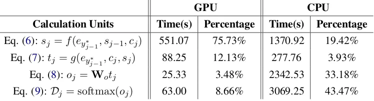
GPU CPU
Calculation Units Time(s) Percentage Time(s) Percentage
Eq. (6):sj =f(ey∗j−1, sj−1, cj) 551.07 75.73% 1370.92 19.42% Eq. (7):tj =g(ey∗
j−1, cj, sj) 88.25 12.13% 277.76 3.93%
Eq. (8):oj =Wotj 25.33 3.48% 2342.53 33.18%
Eq. (9):Dj = softmax(oj) 63.00 8.66% 3069.25 43.47%
Table 1: Time cost statistics for decoding the whole MT03 testset on GPUs and CPUs with beam size10.
which decreased a mass of translation candidates and achieved a significant speed improvement by reducing the size of complicated search space, thereby making it possible to actualize the thought of improving the translation performance through increasing the beam size.
In the traditional SMT decoding, the cube prun-ing algorithm aims to prune a great number of partial translation hypotheses without computing and storing them. For each decoding step, those hypotheses with the same translation rule are grouped together, then the cube pruning algorithm is conducted over the hypotheses. We illustrate the detailed process in Figure1.
3 NMT Decoder with Cube Pruning
3.1 Definitions
We define the related storage unit tuple of the
i-th candidate word in the j-th beam as ni
j =
(ci
j, sij, yij, bpij), where cij is the negative
log-likelihood (NLL) accumulation in the j-th beam,
si
j is the decoder hidden state in thej-th beam,yij
is the index of thej-th target word in large vocab-ulary and bpi
j is the backtracking pointer for the
j-th decoding step. Note that, for each source sen-tence, we begin with calculating its encoded rep-resentation and the first hidden states0
0in decoder,
then searching from the initial tuple(0.0, s0 0,0,0)
existing in the first beam1.
It is a fact that Equation (9) produces the prob-ability distribution of the predicted target words over the target vocabulary V. Cho et al.(2014b) indicated that whenever a target word is generated, thesoftmax function over V computes probabil-ities for all words inV, so the calculation is ex-pensive when the target vocabulary is large. As such, Bahdanau et al. (2015) (and many others) only used the top-30k frequent words as target vocabulary, and replaced others with UNK. How-ever, the final normalization operation still brought high computation complexity for forward calcula-tions.
3.2 Time Cost in Decoding
We conducted an experiment to explore how long each calculation unit in the decoder would take. We decoded the MT03 test dataset by using naive beam search with beam size of 10 and recorded the time consumed in the computation of Equation (6), (7), (8) and (9), respectively. The statistical results in Table1show that the recurrent calcula-tion unit consumed the most time on GPUs, while
1The initial target word indexy0
0equals to0, which
[image:3.595.113.487.238.339.2]the softmax computation also took lots of time. On CPUs, the most expensive computational time cost was caused by thesoftmaxoperation over the entire target vocabulary2. In order to avoid the time-consuming normalization operation in test-ing, we introducedself-normalization(denoted as
SN) into the training.
3.3 Self-normalization
Self-normalization (Devlin et al., 2014) was de-signed to make the model scores which are pro-duced by the output layer be approximated by the probability distribution over the target vocab-ulary without normalization operation. According to Equation (9), for an observed target sentence y = {y∗1,· · ·, y|∗y|}, the Cross-Entropy (CE) loss could be written as
Lθ=−
|y| X
j=1
logDj[yj∗]
=−
|y| X
j=1
log
expoj[y∗j]
P
y0∈V exp (oj[y0])
=
|y| X
j=1
log X
y0∈V
exp oj[y0]
−oj[yj∗]
(10)
where oj is the model score generated by
Equa-tion (8) at the j-th step, we marked the softmax normalizerP
y0∈V exp (oj[y0])asZ.
Following the work ofDevlin et al. (2014), we modified the CE loss function into
Lθ =−
|y| X
j=1
logDj[yj∗]−α(logZ−0)2
=−
|y| X
j=1
logDj[yj∗]−αlog2Z
(11)
The objective function, shown in Equation (11), is optimized to make surelogZ is approximated to0, equally, makeZ close to1once it converges. We chose the value ofαempirically. Because the softmaxnormalizerZ is converged to1 in infer-ence, we just need to ignoreZ and predict the tar-get word distribution at thej-th step only withoj:
Dj =oj (12)
3.4 Cube Pruning
Table 1 clearly shows that the equations in the NMT forward calculation take lots of time. Here, according to the idea behind the cube pruning algorithm, we tried to reduce the time of time-consuming calculations, e.g., Equation (6), and further decrease the search space by introducing the cube pruning algorithm.
3.4.1 Integrating into NMT Decoder
Extended from the naive beam search in the NMT decoder, cube pruning, treated as a pruning al-gorithm, attempts to reduce the search space and computation complexity by merging some simi-lar items in a beam to accelerate the naive beam search, keeping the1-best searching result almost unchanged or even better by increasing the beam size. Thus, it is a fast and effective algorithm to generate candidates.
Assume that T restores the set of the finished translations. For each step in naive beam search process, beamsize−|T| times forward calcula-tions are required to acquirebeamsize−|T| prob-ability distributions corresponding to each item in the previous beam (Bahdanau et al.,2015). while for each step in cube pruning, in terms of some constraints, we merge all similar items in the pre-vious beam into one equivalence class (called a sub-cube). The constraint we used here is that items being merged in the previous beam should have the same target words. Then, for the sub-cube, only one forward calculation is required to obtain the approximate predictions by using the loose hidden state. Elements in the sub-cube are sorted by previous accumulated NLL along the columns (the first dimension of beam size) and by the approximate predictions along the rows (the second dimension of vocabulary size). Af-ter merging, one beam may contain several sub-cubes (the third dimension), we start to search from item in the upper left corner of each sub-cube, which is the best one in the sub-sub-cube, and continue to spread out until enough candidates are found. Once a item is selected, the exact hidden state will be used to calculate its exact NLL.
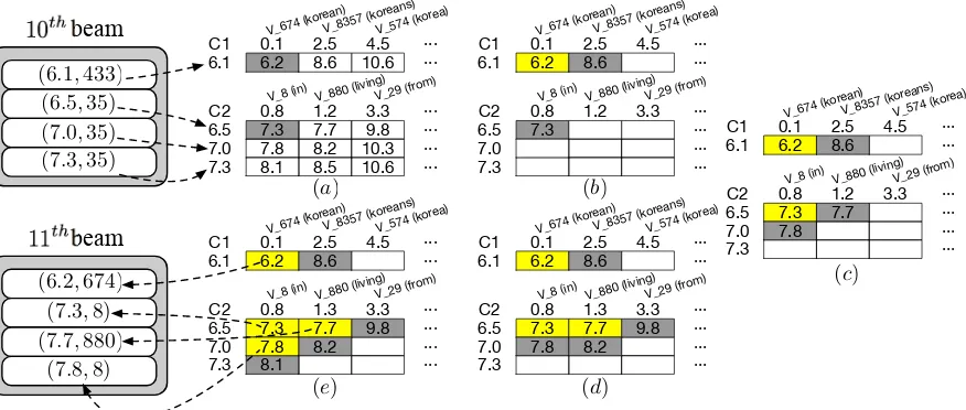
Through all above steps, the frequency of for-ward computations decreases. We give an exam-ple to dive into the details in Figure2.
Assume that the beam size is4. Given the10th
2Note that, identical toBahdanau et al.(2015), we only
0.8 8.1 7.3 7.8 10.6 ··· 7.3 8.5 ··· ··· ··· 10.3 9.8 3.3 1.2 7.7 8.2 7.0 6.5 C2 0.1 6.2 ··· ··· 10.6 4.5 2.5 8.6 6.1
C1 V_674 (kor
ean) V_8357 (kor
eans)
V_574 (kor ea)
V_29 (from) V_880 (living
) V_8 (in)
0.8 7.3 7.8 ··· 7.3 ··· ··· ··· 3.3 1.2 7.7 7.0 6.5 C2 0.1 6.2 ··· ··· 4.5 2.5 8.6 6.1
C1 V_674 (kor
ean) V_8357 (kor
eans) V_574 (kor
ea)
V_29 (from) V_880 (living
) V_8 (in)
0.8 7.3 7.8 ··· 7.3 ··· ··· ··· 9.8 3.3 1.3 7.7 8.2 7.0 6.5 C2 0.1 6.2 ··· ··· 4.5 2.5 8.6 6.1
C1 V_674 (kor
ean) V_8357 (kor
eans)
V_574 (kor ea)
V_29 (from) V_880 (living
) V_8 (in)
0.8 8.1 7.3 7.8 ··· 7.3 ··· ··· ··· 9.8 3.3 1.3 7.7 8.2 7.0 6.5 C2 0.1 6.2 ··· ··· 4.5 2.5 8.6 6.1
C1 V_674 (kor
ean) V_8357 (kor
eans)
V_574 (kor ea)
V_29 (from) V_880 (living
) V_8 (in)
0.8 7.3 ··· 7.3 ··· ··· ··· 3.3 1.2 7.0 6.5 C2 0.1 6.2 ··· ··· 4.5 2.5 8.6 6.1
C1 V_674 (kor
ean) V_8357 (kor
eans)
V_574 (kor ea)
V_29 (from) V_880 (living
) V_8 (in)
(a) (b)
(c)
(d) (e)
beam beam
(6.1,433) (6.5,35) (7.0,35) (7.3,35)
(6.2,674) (7.3,8) (7.7,880)
[image:5.595.78.516.69.255.2](7.8,8)
Figure 2: Cube pruning diagram in beam search process during NMT decoding. We only depict the accumulated NLL and the word-level candidate for each item in the beam (in the bracket). Assume the beam size is4, we initialize a heap for the current step, elements in the10thbeam are merged into two
sub-cubesC1andC2according to the previous target words; (a) the two elements located in the upper-left corner of the two sub-cubes are pushed into the heap; (b) minimal element(6.2,674)is popped out, meanwhile, its neighbor(8.6,8357)is pushed into the heap; (c) minimal element(7.3,8)is popped out, its right-neighbor(7.7,880)and lower-neighbor(7.8,8)are pushed into the heap; (d) minimal element (7.7,880)is popped out, its right-neighbor(9.8,29)and down-neighbor(8.2,880)are pushed into the heap; (e) minimal element(7.8,8)is popped out, then its down-neighbor(8.1,8)is pushed into the heap. 4elements have been popped out, we use them to construct the11th beam. Yellow boxes indicate the
4-best word-level candidates to be pushed into the11thbeam.
beam, we generate the11thbeam. Different from
the naive beam search, we first group items in the previous beam into two sub-cubesC1 andC2 in term of the target word yj−1. As shown in part
(a)of Figure2,(6.1,433)constructs the sub-cube C1; (6.5,35), (7.0,35) and (7.3,35) are put to-gether to compose another sub-cubeC2. Items in part(a)are ranked in ascending order along both row and column dimension according to the ac-cumulated NLL. For each sub-cube, we use the first state vector in each sub-cube as the approx-imate one to produce the next probability distribu-tion and the next state. At beginning, each upper-left corner element in each sub-cube is pushed into a minimum heap, after popping minimum element from the heap, we calculate and restore the exact NLL of the element, then push the right and lower ones alongside the minimum element into heap. At this rate, the searching continues just like the “diffusion” in the sub-cube until 4 elements are popped, which are ranked in terms of their exact NLLs to construct the11th beam. Note that once
an element is popped, we calculate its exact NLL. From the step (e) in Figure 2, we can see that 4
elements have been popped fromC1andC2, and then ranked in terms of their exact NLLs to build the11thbeam.
We refer above algorithm as the naive cube pruning algorithm (calledNCP)
3.4.2 Accelerated Cube Pruning
4 Experiments
We verified the effectiveness of proposed cube pruning algorithm on the Chinese-to-English (Zh-En) translation task.
4.1 Data Preparation
The Chinese-English training dataset consists of 1.25M sentence pairs3. We used the NIST 2002
(MT02) dataset as the validation set with878 sen-tences, and the NIST 2003 (MT03) dataset as the test dataset, which contains919sentences.
The lengths of the sentences on both sides were limited up to50tokens, then actually1.11M sen-tence pairs were left with 25.0M Chinese words and27.0M English words. We extracted30kmost frequent words as the source and target vocabular-ies for both sides.
In all the experiments, case-insensitive 4-gram BLEU (Papineni et al., 2002) was employed for the automatic evaluation, we used the script mteval-v11b.pl4to calculate the BLEU score.
4.2 System
The system is an improved version of attention-based NMT system named RNNsearch (Bahdanau et al., 2015) where the decoder employs a con-ditional GRU layer with attention, consisting of two GRUs and an attention module for each step5. Specifically, Equation (6) is replaced with the fol-lowing two equations:
˜
sj =GRU1(eyj∗−1, sj−1) (13)
sj =GRU2(cj,s˜j) (14)
Besides, for the calculation of relevance in Equa-tion (4), sj−1 is replaced with ˜sj−1. The other
components of the system keep the same as RNNsearch. Also, we re-implemented the beam search algorithm as the naive decoding method, and naive searching on the GPU and CPU server were conducted as two baselines.
4.3 Training Details
Specially, we employed a little different settings from Bahdanau et al. (2015): Word embedding sizes on both sides were set to512, all hidden sizes
3
These sentence pairs are mainly extracted from LDC2002E18, LDC2003E07, LDC2003E14, Hansards por-tion of LDC2004T07, LDC2004T08 and LDC2005T06
4
https://github.com/moses-smt/mosesdecoder/blob/ master/scripts/generic/mteval-v11b.pl
5
https://github.com/nyu-dl/dl4mt-tutorial/blob/ master/docs/cgru.pdf
in the GRUs of both encoder and decoder were also set to512. All parameter matrices, including bias matrices, were initialized with the uniform distribution over[−0.1,0.1]. Parameters were up-dated by using mini-batch Stochastic Gradient De-scent (SGD) with batch size of80and the learning rate was adjusted by AdaDelta (Zeiler,2012) with decay constantρ=0.95 and denominator constant
=1e-6. The gradients of all variables whose L2-norm are larger than a pre-defined threshold 1.0 were normalized to the threshold to avoid gradi-ent explosion (Pascanu et al.,2013). Dropout was applied to the output layer with dropout rate of 0.5. We exploited length normalization (Cho et al.,
2014a) strategy on candidate translations in beam search decoding.
The model whose BLEU score was the high-est on the validation set was used to do thigh-esting. Maximal epoch number was set to 20. Training was conducted on a single Tesla K80 GPU, it took about2days to train a single NMT model on the Zh-En training data. For self-normalization, we empirically setαas0.5in Equation (11)6.
4.4 Search Strategies
We conducted experiments to decode the MT03 test dataset on the GPU and CPU server respec-tively, then compared search quality and efficiency among following six search strategies under differ-ent beam sizes.
NBS-SN:Naive Beam Search withoutSN NBS+SN:Naive Beam Search withSN NCP-SN:Cube Pruning withoutSN NCP+SN:Cube Pruning withSN
ACP-SN: Accelerated Cube Pruning without
SN
ACP+SN:Accelerated Cube Pruning withSN
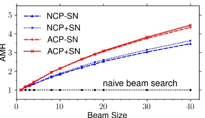
4.5 Comparison of Average Merging Rate
We first give the definition of the Average Merging Rate (denoted as AMR). Given a test dataset, we counted the total word-level candidates (noted as Nw) and the total sub-cubes (noted as Nc) during
the whole decoding process, then the AMR can be simply computed as
m= Nw/Nc (15)
The MT03 test dataset was utilized to com-pare the trends of the AMR values under all
Figure 3: AMR comparison on the MT03 test dataset. Decoding the MT03 test dataset on a sin-gle GeForce GTX TITAN X GPU server under the different searching settings. y-axis represents the AMR on the test dataset in the whole searching process and x-axis indicates beam size. Unsurpris-ingly, we got exactly the same results on the CPU server, not shown here.
six methods. We used the pre-trained model to translate the test dataset on a single GeForce GTX TITAN X GPU server. Beam size varies from 1 to 40, values are included in the set {1,2,3,4,8,10,15,18,20,30,40}. For each beam size, six different searching settings were ap-plied to translate the test dataset respectively. The curves of the AMRs during the decoding on the MT03 test dataset under the proposed methods are shown in Figure3. Note that the AMR values of
NBSare always1whether there isSNor not. Comparing the curves in the Figure3, we could observe that the naive beam search does not con-duct any merging operation in the whole searching process, while the average merging rate in the cube pruning almost grows as the beam size increases. Comparing the red curves to the blue ones, we can conclude that, in any case of beam size, the AMR of the accelerated cube pruning surpasses the ba-sic cube pruning by a large margin. Besides, self-normalization could produces the higher average merging rate comparing to the counterpart without self-normalization.
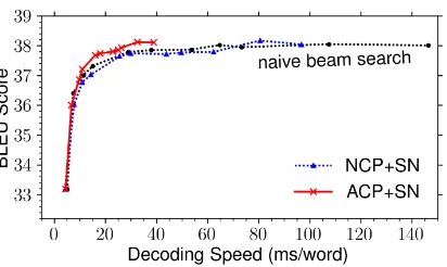
4.6 Comparison on the GPU Server
Intuitively, as the value of the AMR increases, the search space will be reduced and computation ef-ficiency improves. We compare the two proposed searching strategies and the naive beam search in two conditions (with self-normalization and with-out self-normalization). Figure 4 demonstrates the results of comparison between the proposed
searching methods and the naive beam search baseline in terms of search quality and search effi-ciency under different beam sizes.
By fixing the beam size and the dataset, we compared the changing trend of BLEU scores for the three distinct searching strategies under two conditions. Without self-normalization, Figure4a
shows the significant improvement of the search speed, however the BLEU score drops about0.5 points. We then equipped the search algorithm with self-normalization. Figure4bshows that the accelerated cube pruning search algorithm only spend about one-third of the time of the naive beam search to achieve the best BLEU score with beam size30. Concretely, when the beam size is set to be30,ACP+SNis3.3times faster than the baseline on the MT03 test dataset, and both per-formances are almost the same.
4.7 Comparison on the CPU Server
Similar to the experiments conducted on GPUs, we also translated the whole MT03 test dataset on the CPU server by using all six search strate-gies under different beam sizes. The trends of the BLEU scores over those strategies are shown in Figure5.
The proposed search methods gain the similar superiority on CPUs to that on GPUs, and the decoding speed is obviously slower than that on GPUs. From the Figure 5a, we can also clearly see that, compared with the NBS-SN, NCP-SN
only speeds up the decoder a little,ACP-SN pro-duces much more acceleration. However, when we did not introduce self-normalization, the pro-posed search methods will also result in a loss of about 0.5 BLEU score. The self-normalization made the ACP strategy faster than the baseline by about 3.5×, in which condition theNBS+SN
got the best BLEU score 38.05 with beam size 30while theACP+SNachieved the highest score 38.12with beam size30. The results could be ob-served in Figure5b. Because our method is on the algorithmic level and platform-independent, it is reasonable that the proposed method can not only perform well on GPUs, but also accelerate the de-coding significantly on CPUs. Thus, the acceler-ated cube pruning with self-normalization could improve the search quality and efficiency stably.
4.8 Decoding Time
(a) BLEU vs. decoding speed, without self-normalization (b) BLEU vs. decoding speed, with self-normalization
Figure 4: Comparison among the decoding results of the MT03 test dataset on the single GeForce GTX TITAN X GPU server under the three different searching settings. y-axis represents the BLEU score of translations, x-axis indicates that how long it will take for translating one word on average.
[image:8.595.194.507.275.398.2](a) BLEU vs. decoding speed, without self-normalization (b) BLEU vs. decoding speed, with self-normalization
Figure 5: Comparison among the decoding results of the MT03 test dataset on the single AMD Opteron(tm) Processor under the three different searching settings. y-axis represents the BLEU score of translations, x-axis indicates that how long it will take for translating one word on average.
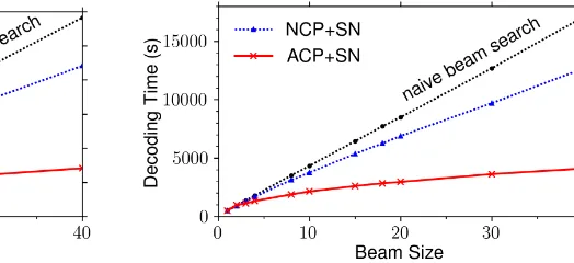
Under the two conditions, we calculated the times spent on translating the entire test dataset for dif-ferent beam sizes, then draw the curves in Figure
6 and 7. From the Figure 6a and 6b, we could observe that accelerated cube pruning algorithm speeds up the decoding by about 3.8×on GPUs when the beam size is set to 40. Figure 7a and
7b show that the accelerated cube pruning algo-rithm speeds up the decoding by about 4.2× on CPU server with the beam size40.
5 Related Work
Recently, lots of works devoted to improve the ef-ficiency of the NMT decoder. Some researchers employed the way of decreasing the target vocabu-lary size.Jean et al.(2015) improved the decoding efficiency even with the model using a very large target vocabulary but selecting only a small sub-set of the whole target vocabulary. Based on the work ofJean et al.(2015),Mi et al.(2016b)
intro-duced sentence-level and batch-level vocabularies as a very small subset of the full output vocabu-lary, then predicted target words only on this small vocabulary, in this way, they only lost0.1 BLEU points, but reduced target vocabulary substantially.
Some other researchers tried to raise the effi-ciency of decoding from other perspectives. Wu et al.(2016) introduced a coverage penaltyα and length normalizationβ into beam search decoder to prune hypotheses and sped up the search pro-cess by30%∼40% when running on CPUs. Hu et al.(2015) used a priority queue to choose the best hypothesis for the next search step, which drastically reduced search space.
phrase-(a) Time spent on translating MT03 test dataset for different beam sizes without self-normalization
[image:9.595.210.507.65.187.2](b) Time spent on translating MT03 test dataset for different beam sizes with self-normalization
Figure 6: Comparison among the decoding results of the MT03 test dataset on the single GeForce GTX TITAN X GPU server under the three different searching settings. y-axis represents the BLEU score of translations, x-axis indicates that how long it will take for translating one word on average.
(a) Time spent on translating MT03 test dataset for different beam sizes without self-normalization
(b) Time spent on translating MT03 test dataset for different beam sizes with self-normalization
Figure 7: Comparison among the decoding results of the MT03 test dataset on the single AMD Opteron(tm) Processor under the three different searching settings. y-axis represents the BLEU score of translations, x-axis indicates that how long it will take for translating one word on average.
based decoding with trigram language model, we can merge states with same source-side coverage vector and same previous two target words). How-ever, this is not appropriate for current NMT de-coding, since the embedding of the previous target word is used as one input of the calculation unit of each step in the decoding process, we could group equivalence classes containing the same previous target word together.
6 Conclusions
We extended cube pruning algorithm into the de-coder of the attention-based NMT. For each step in beam search, we grouped similar candidates in previous beam into one or more equivalence class(es), and bad hypotheses were pruned out. We started searching from the upper-left corner in each equivalence class and spread out until enough
candidates were generated. Evaluations show that, compared with naive beam search, our method could improve the search quality and efficiency to a large extent, accelerating the NMT decoder by 3.3×and3.5×on GPUs and CPUs, respectively. Also, the translation precision could be the same or even better in both situations. Besides, self-normalization is verified to be helpful to accelerate cube pruning even further.
Acknowledgements
[image:9.595.245.507.286.406.2]References
Dzmitry Bahdanau, Kyunghyun Cho, and Yoshua Ben-gio. 2015. Neural machine translation by jointly learning to align and translate. ICLR 2015.
Nicolas Boulanger-Lewandowski, Yoshua Bengio, and Pascal Vincent. 2013. Audio chord recognition with recurrent neural networks. In ISMIR, pages 335– 340. Citeseer.
David Chiang. 2005. A hierarchical phrase-based model for statistical machine translation. In Pro-ceedings of the 43rd Annual Meeting on Association for Computational Linguistics, pages 263–270. As-sociation for Computational Linguistics.
David Chiang. 2007. Hierarchical phrase-based trans-lation. computational linguistics, 33(2):201–228.
Kyunghyun Cho, Bart van Merrienboer, Dzmitry Bah-danau, and Yoshua Bengio. 2014a. On the proper-ties of neural machine translation: Encoder–decoder approaches. InProceedings of SSST-8, Eighth Work-shop on Syntax, Semantics and Structure in Statisti-cal Translation, pages 103–111, Doha, Qatar. Asso-ciation for Computational Linguistics.
Kyunghyun Cho, Bart van Merrienboer, Caglar Gul-cehre, Dzmitry Bahdanau, Fethi Bougares, Holger Schwenk, and Yoshua Bengio. 2014b. Learning phrase representations using rnn encoder–decoder for statistical machine translation. InProceedings of the 2014 Conference on Empirical Methods in Nat-ural Language Processing (EMNLP), pages 1724– 1734, Doha, Qatar. Association for Computational Linguistics.
Jacob Devlin, Rabih Zbib, Zhongqiang Huang, Thomas Lamar, Richard Schwartz, and John Makhoul. 2014. Fast and robust neural network joint models for sta-tistical machine translation. In Proceedings of the 52nd Annual Meeting of the Association for Compu-tational Linguistics (Volume 1: Long Papers), pages 1370–1380, Baltimore, Maryland. Association for Computational Linguistics.
Michel Galley, Jonathan Graehl, Kevin Knight, Daniel Marcu, Steve DeNeefe, Wei Wang, and Ignacio Thayer. 2006. Scalable inference and training of context-rich syntactic translation models. In Pro-ceedings of the 21st International Conference on Computational Linguistics and 44th Annual Meet-ing of the Association for Computational LMeet-inguis- Linguis-tics, pages 961–968, Sydney, Australia. Association for Computational Linguistics.
Jonas Gehring, Michael Auli, David Grangier, and Yann Dauphin. 2017a. A convolutional encoder model for neural machine translation. In Proceed-ings of the 55th Annual Meeting of the Association for Computational Linguistics (Volume 1: Long Pa-pers), pages 123–135, Vancouver, Canada. Associa-tion for ComputaAssocia-tional Linguistics.
Jonas Gehring, Michael Auli, David Grangier, De-nis Yarats, and Yann N. Dauphin. 2017b. Con-volutional sequence to sequence learning. In Pro-ceedings of the 34th International Conference on Machine Learning, volume 70 of Proceedings of Machine Learning Research, pages 1243–1252, In-ternational Convention Centre, Sydney, Australia. PMLR.
Alex Graves. 2012. Sequence transduction with recurrent neural networks. arXiv preprint arXiv:1211.3711.
Sepp Hochreiter and Jrgen Schmidhuber. 1997. Long short-term memory. Neural Computation, 9(8):1735–1780.
Xiaoguang Hu, Wei Li, Xiang Lan, Hua Wu, and Haifeng Wang. 2015. Improved beam search with constrained softmax for nmt. Proceedings of MT Summit XV, page 297.
Liang Huang and David Chiang. 2005. Better k-best parsing. In Proceedings of the Ninth Inter-national Workshop on Parsing Technology, Parsing ’05, pages 53–64, Stroudsburg, PA, USA. Associa-tion for ComputaAssocia-tional Linguistics.
Liang Huang and David Chiang. 2007. Forest rescor-ing: Faster decoding with integrated language mod-els. InProceedings of the 45th Annual Meeting of the Association of Computational Linguistics, pages 144–151, Prague, Czech Republic. Association for Computational Linguistics.
S´ebastien Jean, Kyunghyun Cho, Roland Memisevic, and Yoshua Bengio. 2015. On using very large target vocabulary for neural machine translation. In Proceedings of the 53rd Annual Meeting of the Association for Computational Linguistics and the 7th International Joint Conference on Natural Lan-guage Processing (Volume 1: Long Papers), pages 1–10, Beijing, China. Association for Computa-tional Linguistics.
Nal Kalchbrenner and Phil Blunsom. 2013. Recurrent convolutional neural networks for discourse compo-sitionality. InProceedings of the Workshop on Con-tinuous Vector Space Models and their Composition-ality, pages 119–126, Sofia, Bulgaria. Association for Computational Linguistics.
Haitao Mi, Baskaran Sankaran, Zhiguo Wang, and Abe Ittycheriah. 2016a. Coverage embedding models for neural machine translation. In Proceedings of the 2016 Conference on Empirical Methods in Nat-ural Language Processing, pages 955–960, Austin, Texas. Association for Computational Linguistics.
Franz Josef Och and Hermann Ney. 2004. The align-ment template approach to statistical machine trans-lation. Computational Linguistics, 30(4):417–449.
Kishore Papineni, Salim Roukos, Todd Ward, and Wei-Jing Zhu. 2002. Bleu: a method for automatic eval-uation of machine translation. In Proceedings of 40th Annual Meeting of the Association for Com-putational Linguistics, pages 311–318, Philadelphia, Pennsylvania, USA. Association for Computational Linguistics.
Razvan Pascanu, Tomas Mikolov, and Yoshua Bengio. 2013. On the difficulty of training recurrent neural networks. InProceedings of the 30th International Conference on Machine Learning, volume 28 of
Proceedings of Machine Learning Research, pages 1310–1318, Atlanta, Georgia, USA. PMLR.
Ilya Sutskever, Oriol Vinyals, and Quoc V Le. 2014. Sequence to sequence learning with neural net-works. In Z. Ghahramani, M. Welling, C. Cortes, N. D. Lawrence, and K. Q. Weinberger, editors, Ad-vances in Neural Information Processing Systems 27, pages 3104–3112. Curran Associates, Inc.
Ashish Vaswani, Noam Shazeer, Niki Parmar, Jakob Uszkoreit, Llion Jones, Aidan N Gomez, Ł ukasz Kaiser, and Illia Polosukhin. 2017. Attention is all you need. In I. Guyon, U. V. Luxburg, S. Bengio, H. Wallach, R. Fergus, S. Vishwanathan, and R. Gar-nett, editors, Advances in Neural Information Pro-cessing Systems 30, pages 5998–6008. Curran As-sociates, Inc.
Yonghui Wu, Mike Schuster, Zhifeng Chen, Quoc V Le, Mohammad Norouzi, Wolfgang Macherey, Maxim Krikun, Yuan Cao, Qin Gao, Klaus Macherey, et al. 2016. Google’s neural ma-chine translation system: Bridging the gap between human and machine translation. arXiv preprint arXiv:1609.08144.